2021.06.02.18
Files > Volume 6 > Vol 6 No 4 2021 > Vol 6 No 2 2021
COVID-19 data analysis using HJ-Biplot method: A study case

Franklin Tenesaca-Chillogallo1*, Isidro R. Amaro 2
Available from: http://dx.doi.org/10.21931/RB/2021.06.02.18
ABSTRACT
COVID-19 is a new viral disease declared as a pandemic by the World Health Organization in 2020. This highly infectious disease, caused by the virus Severe Acute Respiratory Syndrome Coronavirus 2 (SARS-CoV-2), has shown a different impact on young individuals, old individuals, and people with other health conditions. In this study, we aim to identify the different relationships between COVID-19 with other health complications. Additionally, our purpose is to ordinate the ages of individuals according to COVID-19 affection. For this, we apply the HJ-Biplot along with Cluster multivariate analysis techniques to a data set of patients diagnosed with COVID-19, Pneumonia, smoking Habits, Diabetes, Obesity, Chronic Obstructive Pulmonary Disease, Asthma, Immunosuppression, Hypertension, Cardiovascular Problems, Chronic Renal Insufficiency, and other health problems. The data set that we use in this work was obtained from the Mexico Government website. This exploratory research illustrates that COVID-19 disease presents different relationships with other health problems and individuals. For example, this viral disease is highly correlated with Hypertension, Diabetes, smoking habits, and Obesity health conditions. Other high correlations are found among Chronic Obstructive Pulmonary Disease, Cardiovascular problems, Pneumonia, Chronic Renal Insufficiency, Hypertension, and Diabetes. Also, the ordination of individuals according to COVID-19 affection shows us that 60 to 89 years old people are highly affected by this disease. Furthermore, we identify the formation of two clusters of individuals.
On the one hand, the first Cluster is formed by old individuals highly affected by many diseases. On the other hand, the second Cluster is formed mainly by young individuals lowly affected by this study's health problems. Identifying COVID-19 correlated health conditions and the age of the most affected individuals is crucial to the correct handle of the pandemic.
Keywords: Cluster, COVID-19, health condition, HJ-Biplot, ordination.
INTRODUCTION
Coronavirus disease 2019 (COVID-19) is a new viral disease that has started spreading from China to the rest of the world since the end of 2019, causing more than 962,600 deaths in approximately 215 countries and territories, as of September 20, 20201,2. This viral disease, caused by the virus Severe Acute Respiratory Syndrome Coronavirus 2 (SARS-CoV-2) has been declared a pandemic by the World Health Organization in February 20202. In this study, our purpose is to understand how health conditions such as Pneumonia, smoking Habits, Diabetes, Obesity, Chronic Obstructive Pulmonary Disease, Asthma, Immunosuppression, Hypertension, Cardiovascular Problems, Chronic Renal Insufficiency are related to COVID-19 disease. Also, we aim to ordinate the ages of individuals according to the impact of COVID-19 disease.
Previous studies performed using data sets from hospitals in Atlanta City and the Shanghai Municipality in the United States and China agrees that old age is a factor risk for COVID-19 condition3–5.
As a methodology, we use the HJ-Biplot Multivariate Analysis Method. This technique provides a two-dimensional space, representing most of the information from the initial data set. The Biplot graph shows the relationship among variables, individuals, and the interactions among variables and individuals in the same reference system. Also, we use Cluster Analysis to discriminate groups of individuals.
The results exposed in this explanatory research may help policymakers in the government make better decisions regarding the management of the health crisis due to the COVID-19 pandemic. This, since we explicitly mention the characteristics of people most affected by this disease. This study case is of particular interest to Mexico since the mortality rate (deaths per 100 confirmed cases) in this country is 10.6%, the highest rate globally as of September 20206.
The paper is organized as follows. In section Materials and Methods, we describe the data and the multivariate methods used in this study. In section Results and Discussion, we present and interpret the results of applying the HJ-Biplot and Cluster methods on the data set. Finally, in section Conclusions, we state the reasoned judgments obtained from this study.
MATERIALS AND METHODS
Data General Description
The data set used in this study was obtained from the online page of the Government of Mexico7. This data source provides public information regarding COVID-19 spread in Mexico. In the original data set, 35 variables collect general information of
In this study, we consider only the variables that are related to diseases and other health conditions. In total, we use 12 variables, which are explained in Table 1. At the same time, we considered 12 groups of age to the analysis; the groups' characteristics are explained in Table 2.
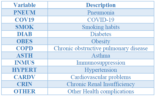
Table 1. Variables Description.
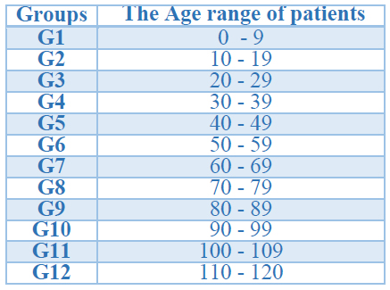
Table 2. Groups Description.
Table 3 shows the number of positive infected people in each group for each variable. However, we see that these values change enormously along rows, and therefore multivariate analysis techniques would not allow us to interpret the data correctly. This problem is fixed by creating a relative data set, i.e., each element in the new Relative Data Set shows the proportion between the number of positive cases and the number of patients for each group and variable. The data set containing the relative values is shown in Table 4.
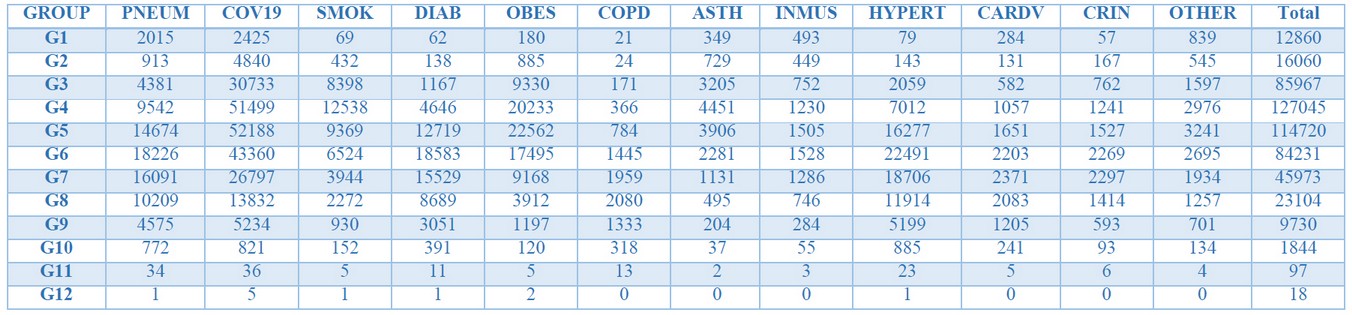
Table 3. Absolute values Table.
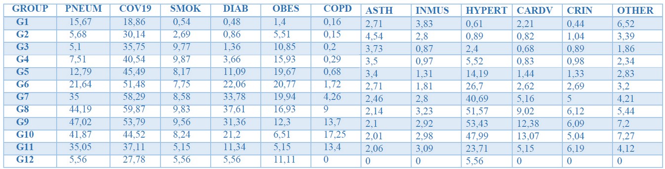
Table 4. Relative values Table.
HJ-Biplot Method
Biplot is a multivariate analysis technique developed by Gabriel 19718. This method permits the representation of X (I*J data matrix) in a low dimensional space facilitating its interpretation. This procedure is accomplished by the simultaneous representation of row and column markers a1,a2,…aI and b1,b2,…bI respectively. These row and column markers are obtained with help of the Singular Value Decomposition (SVD) of the data matrix X . Thus, we write:

where U is the matrix whose columns are the eigenvectors of XXT,D is the matrix whose diagonal elements contain the singular values of X is the matrix whose columns are the eigenvectors of XTX. Then, we choose A(I*S matrix) and B (S*J matrix) such that:

and the Xij element of X A = U and , BT = VD and JK-Biplot where A= UD and BT = V
In the current project, we use the HJ-Biplot method with Singular Value Decomposition. In this reference system, rows and columns in X are illustrated with the highest quality of representation. In the HJ-Biplot case, the properties of row markers are similar to those in the JK-Biplot, and the properties of the column markers are similar to those in the GH-Biplot10,11.
Properties of the HJ-Biplot
1. Both Row and Column markers are represented simultaneously in a Euclidean space with the same highest representation quality.
2. The scalar product of the columns of X is equal to the scalar product of the column markers.

3. The scalar product of the rows in X
4. The length of the vector representing the variable Xj is proportional to the variance of that variable.
5. The cosine of the angle between two vectors bi and bj representing the variables Xi and Xj
6. The Mahalanobis distances between individuals are interpreted as inverse similarities. Hence, these distances are approximated by the row markers' Euclidean distances (representing the groups of age). Hence,

where Σ is an estimate of the corresponding variance-covariance matrix.
7. The projections of row markers (points) onto the column markers (arrows) allow individuals' ordination regarding its value in the variables.
Graphical interpretation of HJ-Biplot
For column markers: The length of a column marker (vector) bj representing the variable Xj is proportional to the variance of that variable; in this sense, longer column vectors show greater variance than shorter column vectors. Also, the cosine of the angle between the column vectors bi and bj approximate the correlation between the variables Xi and Xj . Therefore, vectors forming angles less than 90o justify a high positive correlation between the represented variables; 90o or close angles show that there is no correlation; 180o or close angles evidence a high negative correlation between variables Xi and Xj .
For row markers: The distance between row markers (points) represents an inverse similarity because closer individuals are more similar than the distant ones. This property allows the formation of clusters of individuals in our graph.
For projections of row markers onto column markers: The order of the projections of row markers (points) onto column markers (arrows) approximates each individual's value onto that variable. Hence, the values of the individuals whose projections fall near to the origin are close to the mean value of that variable. The values of the individuals whose projections fall away from the origin and in the same direction of the column marker are large. The values of the individuals whose projections fall away from the origin but on the other direction of the column marker are small.
Since biplots' characteristics allow researchers in different fields to interpret high dimensional sets of data, it has been used in enology, mycology, image analysis, genetics, hydrology, botany, decision theory, library science, and ecology. Specifically, the HJ-Biplot method has been applied in immunology, entomology, enology, geology, marine biology, and sociology. A more exhaustive review of HJ-Biplot applications can be found in Nieto 201411. Some recent applications of the HJ-Biplot method are found in Serafim 201310; Gallego-Álvarez 2015 12; Delgado-Álvarez 2015 13; Patino-Alonso 201514; Hernández-Suárez 201615; Ruiz 201816; Oliveira-Da Silva 201917; and Jaramillo-Feijoo 202018.
Hierarchical clustering
Cluster analysis is a set of numeric techniques that create clusters or groups of elements with similar characteristics19. In hierarchical clustering, the elements are grouped following some steps that may start from a cluster for each of the classified elements and end up with a single cluster containing all the elements. Hierarchical methods are classified as agglomerative and divisive techniques. Some agglomerative hierarchical clustering methods are average linkage, complete linkage, single linkage, ward linkage, weighted linkage, median linkage, and centroid linkage, all operating similarly20,21. Each of these techniques has a cophenetic matrix and a dendrogram (or tree diagram) associated. One way to compare these methods' performance is by contrasting the cophenetic correlation coefficient (CPCC) obtained from each matrix. In this sense, the best hierarchical clustering method is the one with the highest CPCC. Previous studies have shown that the average and centroid linkage methods with Euclidean distance measure are the best techniques for hierarchical agglomerative clustering21.
Another relevant aspect of hierarchical clustering is the number of clusters to be chosen. In this regard, the number of clusters is determined using the dendrogram. Hence, we place a line at a certain height of the dendrogram identifying the number of clusters formed below. To place the line (or best cut) at the most convenient height on the dendrogram, some researchers have proposed methods such as the static tree cut, dynamic tree cut, and others20,22,23. However, there is not a fixed criterion regarding which method gives the appropriate number of clusters. Oldham 2006 has shown that the static tree cut method is the most helpful technique in a hierarchical configuration24. The static tree cut technique proposes the line's placement on the dendrogram at the most significant space between two fusion levels (the heights in the dendrogram where the clusters form)20. In our dendrogram, we place the line approximately at the height of 4.5. This, since between the two fusion levels close to the heights 4 and 5, there are no changes in the number of clusters. In this way, we differentiate 2 clusters. Further applications of clusters are detailed in Everitt 201120. Some recent uses of cluster analysis are found in Serafim 201310; Patino-Alonso 201514; Jaramillo-Feijo 202018; and Zhang 202025.
RESULTS AND DISCUSSION
In this exploratory study, we have started with a data set of 35 variables and 595917 individuals. Then, we have focused on 12 variables related to diseases and health conditions, including COVID-19. Also, we have classified the individuals into 12 different groups according to age. Both variables and group details are shown in Tables 1 and 2, respectively. After that, we have created a table of relative values (Table 4) used in the MultBiplot statistical software26. The results of this application are presented and discussed below.
In Table 5, we present the eigenvalues, inertias, and cumulative inertias for our HJ-Biplot. We see that our matrix X is well represented by the first two axes accounting for 82.17% of the total inertia.
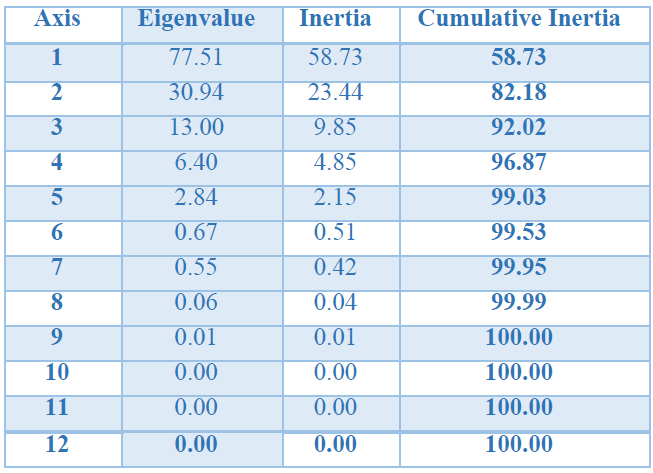
Table 5. Eigenvalues, Inertias, and Cumulative Inertias of HJ-Biplot.
In Figure 1, we have the HJ-Biplot representation of the groups and variables on the same reference system through the row and column markers. In this two-dimensional plot, we consider the relative values (Table 4) instead of the absolute ones (Table 3). Moreover, we discriminate the groups of individuals with two clusters using the average linkage hierarchical clustering method (CPCC = 0.7729) which has proven to be better than centroid linkage (CPCC = 0.7694), complete linkage (CPCC = 0.7663), median linkage (CPCC = 0.7556), ward linkage (CPCC = 0.7534), weighted linkage (CPCC = 0.7253), and single linkage (CPCC = 0.6729) methods. The number of clusters is obtained with the use of the static tree cut method. Hence, in Figure 2, we see the dendrogram with the corresponding best cut (red line) at the height of 4.5, evidencing the formation of two clusters.
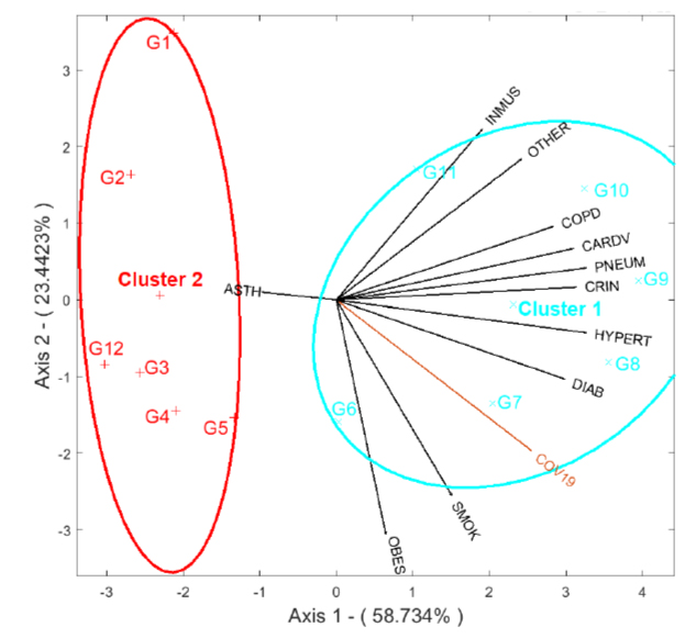
Figure 1. HJ-Biplot of groups and variables.
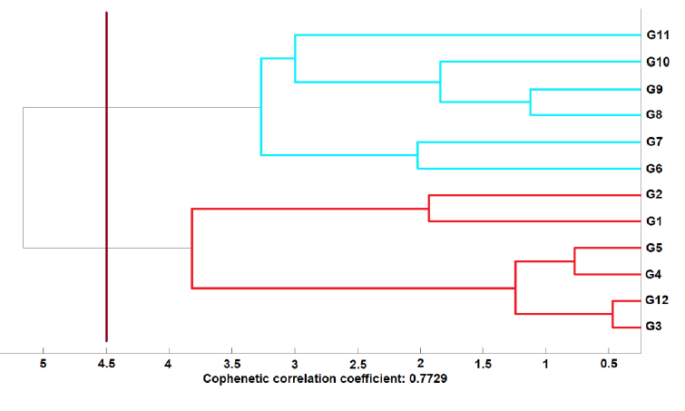
Figure 2. Dendrogram of the hierarchical Cluster with average linkage.
We consider that a marker has a sufficiently high quality of representation on this graph if its value is more significant than half of the value of the best-represented column or row marker27. From this perspective, in Table 6, we have the quality of representation of each axis's variables. On the one hand, we see that the correctly interpreted variables are PNEUM, COV19, SMOK, DIAB, OBES, COPD, INMUS, HYPERT, CARDV, CRIN, and OTHER since they meet our criteria for a sufficiently high quality of representation. On the other hand, the variable ASTH does not achieve a sufficiently high quality of representation, and therefore we cannot interpret this variable in our two-dimensional space.
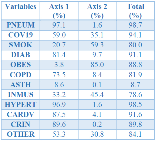
Table 6. Quality of representation for variables.
Also, in Table 7, we show the quality of representation of each group on the plot. Following the same criteria as before we see that all groups have a high quality of representation on this plot. This leads us to a correct interpretation of all groups in two dimensions.
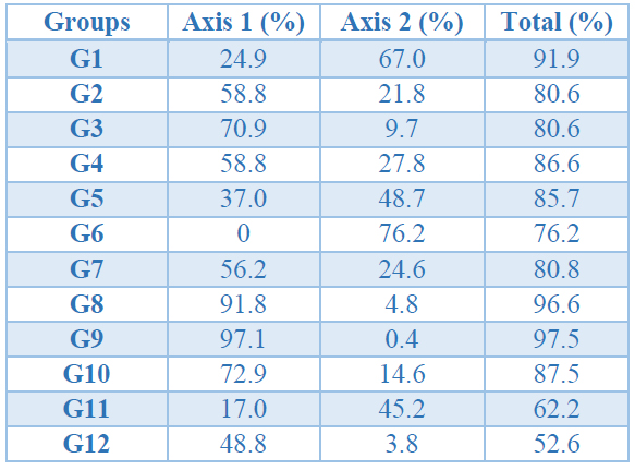
Table 7. Quality of representation for groups.
By the HJ-Biplot properties mentioned above, the variables represented by vectors forming angles close to 0° among them are positively highly correlated. For example, the variable COV19 has a strong positive correlation with HYPERT, DIAB, SMOK, and OBES. Similarly, we find other correlated variables such as INMUS and OTHER; SMOK and OBES; COPD, CARDV, PNEUM, CRIN, HYPERT, and DIAB. Whereas the variables forming angles close to 180° are negatively highly correlated. For instance, INMUS and OBES. Meanwhile, the variables represented by vectors forming angles close to 90° among them are minor or uncorrelated. For instance, the variable COV19 has a small or no correlation with the variables INMUS and OTHER. Other examples of uncorrelated variables are INMUS and DIAB; COPD and OBES; COPD and SMOK; CARDV and OBES; CARDV and SMOK; PNEUM and OBES; PNEUM and SMOK; CRIN and OBES; CRIN and SMOK; HYPERT and OBES. Recall that the variable ASTH cannot be correctly interpreted in this biplot.
Also, by the previously mentioned properties, the vectors' length representing the variables approximate its variance. Therefore, INMUS, OTHER, COPD, CARDV, PNEUM, CRIN, HYPERT, DIAB, COV19, SMOK, and OBES have similar variances.
The arrangement of groups (individuals) in the factorial plane is also interpreted, given the HJ-Biplot properties. Figure 1 evidences the presence of two clusters. Cluster 1 (right side of the graph) comprises older adults G6, G7, G8, G9, G10, and G11. Cluster 2 (left side of the graph) comprises young individuals G1, G2, G3, and G4. The groups G3, G4, and G5 are closer than other groups indicating a similar behavior regarding the studied variables.
In Figure 3, we see the projections of the groups (individuals) onto the vector of the variable COV19, which is one of the main motivations for our study. In this graph, the projections are labeled with the group's name, preceded by the letter "P" (for example, PG1 is the projection of G1 onto the column marker COV19). We observe an ordination of the projections onto the variable COV19 according to the values these groups have in that variable. On the one hand, we observe that most of the proportion of patients affected by COVID-19 are in the groups G7, G8, and G9, i.e., 60 to 89 years old. On the other hand, the minor proportion of people affected by this disease are in the groups: G1 and G2, i.e., they are 0 to 19 years old. The groups G1, G2, G12, G3, G4, and G5 have low values on the variables COPD, CARDV, PNEUM, CRIN, HYPERT, DIAB, and COV19. While the groups G7, G8, G9, and G10 have high values on the same variables. These results are concordant with other investigations reported in Killerby 20203; Li 20204; The Novel Coronavirus Pneumonia Emergency Response Epidemiology Team 20205. A similar analysis can be performed with the rest of the groups and variables plotted in our graph.
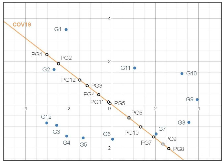
Figure 3. Projections of groups onto the variable COV19.
CONCLUSIONS
The HJ-Biplot application to our data set is helpful because of its visual interpretability. This feature allows the visual exploration and analysis of correlations among the variables associated with diseases and other health conditions and reflects the information of these variables in relation to each group. It also makes an ordination of groups according to its value in each variable. Moreover, the quality of representation of column and row markers on this biplot is high. This, since all groups and 11 out of 12 variables are highly represented on this graph.
We find that patients affected by the COVID-19 disease share some common characteristics. For example, we see that people that get sick with the COVID-19 disease are also affected by Hypertension, Diabetes, smoking habits, and the Obesity health condition. Additionally, the age of the patients plays an important role, being it another critical characteristic. In this sense, the groups' ordination over the variable of COVID-19 shows that the most affected patients are 60 to 89 years old and that the less affected individuals are 0 to 19 years old. Furthermore, the configuration of groups on this biplot shows two main clusters. We see that most of the first Cluster groups represent older people while most of the second Cluster groups represent young patients.
There are other relations among variables and among groups and other interactions among variables and groups that result from this study. These relationships are interpreted similarly. For instance, in this two-dimensional space, we find a correlation among variables representing Chronic Obstructive Pulmonary Disease, Cardiovascular problems, Pneumonia disease, Chronic Renal Insufficiency, Hypertension, and Diabetes. Also, regarding the ordination of groups over the variables, we see that most of the groups representing young people have low values on the previously indicated variables, while groups representing older adults have high values on the same variables. In general, these findings suggest that older individuals are more related to the diseases and health conditions mentioned earlier than younger people.
The results presented in this explanatory paper state a precedent for future investigations from a medical approach. Specifically, it is necessary to investigate the implications of the different grades of correlation among variables, groups, and between variables and groups. Another improvement for this paper could be acquired by using variables representing other relevant health conditions.
REFERENCES
1. Worldometer. Coronavirus Cases [Internet]. Worldometer. 2020 [cited 2020 Sep 20]. p. 1–22. Available from: https://www.worldometers.info/coronavirus/?
2. World Health Organization. Report of the WHO-China Joint Mission on Coronavirus Disease 2019 (COVID-19) [Internet]. Vol. 1, The WHO-China Joint Mission on Coronavirus Disease 2019. 2020. Available from: https://www.who.int/docs/default-source/coronaviruse/who-china-joint-mission-on-covid-19-final-report.pdf
3. Killerby ME, Link-Gelles R, Haight SC, Schrodt CA, England L, Gomes DJ, et al. Characteristics Associated with Hospitalization Among Patients with COVID-19-Metropolitan Atlanta, Georgia, March-April 2020 [Internet]. Metropolitan Atlanta, Georgia; 2020 Jun [cited 2020 Aug 11]. Available from: https://www.cdc.gov/coronavirus/2019-ncov/hcp/infection-control-
4. Li X, Xu S, Yu M, Wang K, Tao Y, Zhou Y, et al. Risk factors for severity and mortality in adult COVID-19 inpatients in Wuhan. J Allergy Clin Immunol [Internet]. 2020 July 1 [cited 2020 August 11];146(1):110–8. Available from: https://www.sciencedirect.com/science/article/pii/S0091674920304954
5. The Novel Coronavirus Pneumonia Emergency Response Epidemiology Team. The Epidemiological Characteristics of an Outbreak of 2019 Novel Coronavirus Diseases (COVID-19) — China, 2020. China CDC Wkly [Internet]. 2020 Feb 1 [cited 2020 Sep 20];2(8):113–22. Available from: http://weekly.chinacdc.cn/en/article/doi/10.46234/ccdcw2020.032
6. Johns Hopkins University. Mortality Analyses - Johns Hopkins Coronavirus Resource Center [Internet]. 2020 [cited 2020 Aug 2]. Available from: https://coronavirus.jhu.edu/data/mortality
7. Gobierno de México. Datos Abiertos de México - Información referente a casos COVID-19 en México - Bases de datos COVID-19 [Internet]. 2020 [cited 2020 Aug 2]. Available from: https://datos.gob.mx/busca/dataset/informacion-referente-a-casos-covid-19-en-mexico/resource/e8c7079c-dc2a-4b6e-8035-08042ed37165?inner_span=True
8. Gabriel KR. The biplot graphic display of matrices with application to principal component analysis. Biometrika [Internet]. 1971 Dec 1 [cited 2020 Sep 14];58(3):453–67. Available from: https://academic.oup.com/biomet/article/58/3/453/233361
9. Galindo M. Una alternativa de representación simultánea: HJ-Biplot [Internet]. 1986 [cited 2020 Aug 25]. p. 13–23. Available from: https://www.researchgate.net/publication/39430983_Una_alternativa_de_representacion_simultanea_HJ-Biplot
10. Serafim A, Company R, Lopes B, Silva N, Castela E, Bebianno MJ, et al. Profile analysis of mothers susceptible to contaminant exposure in the Algarve region: Application of the HJ-BIPLOT method. Biometrical Lett [Internet]. 2013 Aug 19 [cited 2020 Sep 14];49(1):57–66. Available from: https://content.sciendo.com/view/journals/bile/49/1/article-p57.xml
11. Nieto AB, Galindo MP, Leiva V, Vicente-Galindo P. Una metodología para biplots basada en bootstrapping con R. Rev Colomb Estad. 2014;37(2):367–97.
12. Gallego-Álvarez I, Galindo-Villardón MP, Rodríguez-Rosa M. Analysis of the Sustainable Society Index Worldwide: A Study from the Biplot Perspective. Soc Indic Res. 2015;120(1):29–65.
13. Delgado Álvarez JF, Villardon PG. A proposal for spatio-temporal analysis of traffic matrices using HJ-biplot. 2015 IEEE Int Work Meas Networking, M N 2015 - Proc. 2015;(1):88–93.
14. Patino-Alonso MC, Recio-Rodríguez JI, Magdalena-Belio JF, Giné-Garriga M, Martínez-Vizcaino V, Fernández-Alonso C, et al. Clustering of lifestyle characteristics and their association with cardio-metabolic health: The Lifestyles and Endothelial Dysfunction (EVIDENT) study. Br J Nutr. 2015 Aug 13;114(6):943–51.
15. Hernández Suárez M, Molina Pérez D, Rodríguez-Rodríguez E, Díaz Romero C, Espinosa Borreguero F, Galindo-Villardón P. The Compositional HJ-Biplot—A New Approach to Identifying the Links among Bioactive Compounds of Tomatoes. Int J Mol Sci [Internet]. 2016 Nov 2 [cited 2020 Sep 16];17(11):1828. Available from: http://www.mdpi.com/1422-0067/17/11/1828
16. Ruiz NC, Egido J, Galindo-Villardón P, Del-Río P. Advantages of using HJ-Biplot analysis in executive functions studies. Psicol Teor e Pesqui. 2018;34:1–8.
17. Oliveira Da Silva A, Freitas A. The HJ-Biplot Visualization of the Singular Spectrum Analysis Method. 2019.
18. Jaramillo Feijo LE, Galindo Villardon MP, Real Cotto JJ. Análisis clúster para big data: una aplicación con variables demográficas en provincias del Ecuador Cluster analysis for big data: an application with demographic variables in provinces of Ecuador. Vol. 6, J. health med. sci. 2020.
19. Everitt BS, Hothorn T. A handbook of statistical analyses using R. 2nd ed. 2010.
20. Everitt BS, Landau S, Leese M, Stahl D. Cluster Analysis. 2011.
21. Saraçli S, Doǧan N, Doǧan I. Comparison of hierarchical cluster analysis methods by cophenetic correlation. J Inequalities Appl [Internet]. 2013 Apr 23 [cited 2020 Sep 24];2013(1):1–8. Available from: https://link.springer.com/articles/10.1186/1029-242X-2013-203
22. Milligan GW, Cooper MC. An examination of procedures for determining the number of clusters in a data set. Psychometrika [Internet]. 1985 Jun [cited 2020 Sep 25];50(2):159–79. Available from: https://link.springer.com/article/10.1007/BF02294245
23. Langfelder P, Zhang B, Horvath S. Defining clusters from a hierarchical cluster tree: The Dynamic Tree Cut package for R. Bioinformatics [Internet]. 2008 Mar 1 [cited 2020 Sep 25];24(5):719–20. Available from: https://academic.oup.com/bioinformatics/article/24/5/719/200751
24. Oldham MC, Horvath S, Geschwind DH. Conservation and evolution of gene coexpression networks in human and chimpanzee brains. Proc Natl Acad Sci U S A [Internet]. 2006 Nov 21 [cited 2020 Sep 25];103(47):17973–8. Available from: www.pnas.orgcgidoi10.1073pnas.0605938103
25. Zhang J, Cao Y, Tan G, Dong X, Wang B, Lin J, et al. Clinical, radiological, and laboratory characteristics and risk factors for severity and mortality of 289 hospitalized COVID‐19 patients. Allergy [Internet]. 2020 Aug 24 [cited 2020 Sep 19];all.14496. Available from: https://onlinelibrary.wiley.com/doi/abs/10.1111/all.14496
26. José Luis Vicente Villardón. MULTBIPLOT: A apackage for Multivariate Analysis using Biplots. [Internet]. 2016. Available from: http://biplot.usal.es/ClassicalBiplot/index.html
27. González Cabrera JM, Fidalgo Martínez MR, Martín Mateos EJ, Vicente Tavera S. Study of the evolution of air pollution in Salamanca (Spain) along a five-year period (1994-1998) using HJ-Biplot simultaneous representation analysis. Environ Model Softw. 2006 Jan 1;21(1):61–8.
Received:10 November 2020
Accepted: February 15 2021
Franklin Tenesaca-Chillogallo1*, Isidro R. Amaro 2
1. School of Mathematical and Computational Sciences. Yachay Tech University. Ecuador.
https://orcid.org/0000-0002-6308-6652
Corresponding Author: [email protected]
2. Professor. School of Mathematical and Computational Sciences. Yachay Tech University. Ecuador.
https://orcid.org/0000-0003-2402-910x