2023.08.01.45
Files > Volume 8 > Vol 8 No 1 2023
A model for the SARS-CoV-2 dynamics in a population lacking herd immunity

Paúl Medina-Vásquez 1* , Ray Romero-Romero2 and Juan Mayorga-Zambrano 2,
1 Universidad de las Fuerzas Armadas ESPE;
2 Yachay Tech University; [email protected]; [email protected]
Corresponding author. [email protected]
Available from: http://dx.doi.org/10.21931/RB/2023.08.01.45
ABSTRACT
We introduced the S-HI model, a generalized SEIR model to describe the dynamics of the SARS-CoV-2 virus in a community without herd immunity and performed simulations for six months. The S- HI model consists of eight equations corresponding to susceptible individuals, exposed, asymptomatic infected, asymptomatic recovered, symptomatic infected, quarantined, symptomatic recovered and dead. We study the dynamics of the infected, asymptomatic. Dead classes in 4 different networks: households, workplaces, agglomeration places and the general community, showing that the dynamics of the three compartments have the exact nature in each layer and that the speed of the disease considerably increases in the networks with the highest weight of contacts. The reproduction number, R0, is greater than 1 in all networks conforming to the theory. The variants of the SARS-Cov-2 virus are not taken into account, so the S-HI model would fit a situation similar to the first wave of contagion after the mandatory lockdown.
Keywords: SARS-Cov-2, mathematical models, SEIR, data-driven networks, simulations, basic reproduction number, lack of herd immunity.
INTRODUCTION
Herd immunity is usually desirable to confront an epidemic, i.e., an infectious disease that affects many members within a population in a specific area. Herd immunity is presented when most of a population is immune to an infectious disease, providing protection even to individuals - like newborns - that are not immune.1 This can be achieved, for example, when enough people have been vaccinated against the disease; this principle has worked well against diphtheria, smallpox, etc., and it's currently declared by governments as a goal to fight the current SARS-CoV-2 (severe acute respiratory syndrome coronavirus 2) epidemic.
With some exceptions, communities from developed countries are paving their way to get herd immunity. To keep it, they have even started to apply a third booster dose and have created vaccination programs for children 2-6 years old. On the other side, in general, underdeveloped countries, because of economic restrictions or faults in managing or even corruption, have not been able to design and successfully apply mass vaccination plans and, consequently, are very far from ob- obtaining herd immunity. No more than 2% of people in these countries have received at least one dose; this has consequences for public health and economic limitations for individual citizens.1 This particular situation of most undeveloped countries, where many people make their living daily, makes it almost impossible for the governments to apply new total lockdown measures for long periods as it was done at the beginning of 2020.
The first epidemiological model dates back to 1766 when D. Bernoulli used mathematical methods to analyze the behavior of smallpox.2 Modern Mathematical Epidemiology started with the first compartmental model to study the spreading of infectious diseases. In 1927 Kermack and McKendick presented the SIR model, a deterministic machinery that distinguishes three classes of individuals: susceptible, infected and recovered.3 The current SARS-CoV-2 epi- demic dynamics have been modeled by extending the standard SEIR model, adding a class of exposed individuals.4 For us, papers 4-6 were the primary sources of motivation to model the SARS-CoV-2 dynamics in a population lacking herd immunity like most underdeveloped countries.
Although6 does not study the current outbreak of SARS-CoV-2, it helps to understand how the dynamics of a spread disease change in different contact networks and, therefore, is helpful to perform more accurate predictions.
The models built in4 and5 didn't consider demographic characteristics, so deaths not directly caused by SARS-CoV-2 are not considered. We follow this criterion in the model we introduce in this paper.
The work5 studies the effect of lockdown measures on the pandemic dynamics. Unlike other models, where the quarantined population is considered a separate compartment, in5, the characteristic is reflected in the time-dependent contagion factor, β.
On the other hand,4 considers the population subjected to isolation as an individual class. It focused on a scenario where quarantine is mandatory only for the infected people. The approach of6 somehow complements this paper because the latter analyzes and places a specific weight on the different places of agglomeration: schools, workplaces, households and the general community.
This paper presents a new model motivated by works4-6, referred to as S-HI (SARS-CoV-2 without herd immunity) model. It aims to abstract the SARS-CoV-2 dynamics in the context of the so-called "new normality" of communities or countries which have not attained herd immunity and that, unfortunately, are far from getting it. As was already mentioned, to build the S- HI model, we assume, as do4 and5, that demographic constraints are irrelevant: the deaths not directly caused by SARS-CoV-2 do not affect its dynamics.
We differentiate two infectious classes: asymptomatic infected and symptomatic infected. Since asymptomatic infected individuals are hard to track, we only consider the population in the symptomatic infected compartment to be isolated. All the asymptomatic individuals will become asymptomatic and recover at a specific rate. Also, we believe the social distance and the use of masks as a mitigation of the transmission rate, β. Every parameter is obtained as the inverse of an individual's average time period in a single class.
MATERIALS AND METHODS
Remark 1.1. Further studies can consider a vaccinated class. This could help study the SARS- CoV-2 dynamics in communities or countries that have vaccinated a considerable portion of its population but are still far from getting herd immunity.
The S-HI model, presented in Section 2, consists of eight ordinary differential equations corresponding to the following classes of individuals: susceptible, exposed, asymptomatic infected, asymptomatic recovered, symptomatic infected, quarantined, recovered and dead. Although in this work, we take β, the transmission rate, as a constant, it is essential to emphasize that a more in-depth study of this factor can be carried out and would lead to a more precise representation of the situation under consideration.
In our simulations, presented in Section 3, we consider the dynamics of SARS-CoV-2 in 4 different layers: general community, households, workplaces and agglomeration places. In each of these places, the symptomatic infected curve shows an other behavior reflected in the speed to reach its peak. The computation of the reproduction number, R0, is obtained as the spectral value of the next-generation matrix. Although R0 barely differs between layers, this value is greater than 1 in each situation, a fact compatible with the theory.
S-HI model
In this section, we introduce the S-HI model, which, as mentioned in Section 1, is motivated by works4-6. We consider eight individual classes (see Figure 1) and denoted by
𝑆(𝑡), 𝐸(𝑡), 𝐴(𝑡), 𝑉(𝑡), 𝐼(𝑡), 𝑄(𝑡), 𝑅(𝑡) and 𝐷(𝑡), respectively, the number of susceptible, exposed, asymptomatic infected, asymptomatic recovered, symptomatic infected, quarantined, symptomatic recovered and dead individuals at a time t in an interval of study [0,T], T > 0.

Figure 1. Flowchart of the S-HI model.
To begin with, we shall assume that T is not significant and, therefore, as in4 and5, we discard demographic constraints. This implies that the size of the population is constant:

We deal with a fully-susceptible population that can move to the exposed class by interacting with two compartments of infectious individuals: asymptomatic and symptomatic infected. A latent period of around 𝜎−1 𝜖 [2,3] days follows after an individual becomes exposed5. After this period, the individual can become either asymptomatic or symptomatic infected. The asymptomatic path is much simpler as these persons don't even realize that they are not infected. The asymptomatic infectious period, 𝑀−1, is typical of 7 days. Symptomatic infected individuals become quarantined at rate δ. This isolation usually lasts 14 days.7 The death rate of isolated individuals shall be denoted by κ.
The transmission rate usually denoted β, is the interaction factor that leads to new infectious. We indicate βSA, the corresponding value for the interaction between susceptible and asymptomatic individuals and by βSI, the value for the exchange of susceptible and symptomatic individuals. The rates of cure or recovery, λ(𝑡), and mortality, κ(𝑡), are taken as proposed in4. The remaining parameters are kept constant. Then the equations of the model are

The S-HI model works under the following assumptions:
· the number of births and deaths in the period considered does not affect the size of the population;
· no one enters or leaves the people; it is closed;
· recovered individuals obtain immunity; they cannot get infected by the disease again.
Individuals in the isolated class do not participate in the total active population dynamics. That is the reason why the total active population in the denominator of the standard incidence is N-Q.
RESULTS
As in5,7-9, we have that the transmission rate, whether from contact with asymptomatic infected or symptomatic infected individuals, is very close to 1; the latent period is about 2-3 days, so 𝜎−1𝜖[2,3]; the total incubation period is of 4-7 days, then 𝛾−1𝜖 [4,7]; the time scale of recovery for asymptomatic is seven days, therefore 𝑀−1 = 7; also, the time scale of going from infected class to isolated compartment 𝛿 = 0101. To compatibilized with the theory, we produced several numerical experimentations that led us to fix the parameters as follows:

Isolated individuals are expected to recover at rate λ(𝑡) and die at rate κ(𝑡), and they are taken as in.4 The cure rate 𝜆(𝑡) gradually increases with time, while the death rate rapidly de- creases in the same period; this phenomenon is due to the newness of the disease; as time progresses, new and more effective treatments are discovered to control the disease.4 The system is rewritten as 𝑌′(𝑡) = 𝐴𝑌(𝑡) + 𝐾 + 𝐺, where
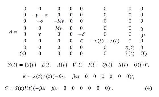
where 𝑍∗ denotes the transposed of the matrix 𝑍. The system is solved by the fourth-order Runge-Kutta method, working as in.10

Figure 2. Dynamics of the S-HI model within a population of 17 million people.
In Figure 2 we see the expected dynamics of the SARS-CoV-2 virus simulated by the S-HI model. The susceptible curve decreases as fast as the asymptomatic and symptomatic curves reach their peaks. The model predicts a scenario where the last isolated individuals will be disease-free in about five months.
Remark 3.1. Unfortunately, our results could not fit the underdeveloped data governments have made public, mainly because of their lack of transparency. We must also note that we are not taking into account the disobedience in bio-safety issues by a segment of the population, and neither are we taking into account the variants of the SARS-Cov-2 virus. Therefore, the S-HI model would fit, for example, the situation corresponding to the first wave of contagion after the mandatory lockdown.
We fix the contact weights of the four layers as in.6. Then we put 0.18 and 0.33. 0.3 and 0.19 for the general community, households, workplaces, and agglomeration places, respectively. It is im- essential to mention that we consider the same pack of initial values in every network. These contact weights influence the transmission rates, βSA and βSI, which are computed as 𝛽𝑆𝐴 = 𝜔𝑙 ∗ 𝜌𝑆𝐴 and
𝛽𝑆𝐼 = 𝜔𝑙 ∗ 𝜌𝑆𝐼 where ρ is the probability of transmission per contact, 1/𝑑𝑎𝑦𝑠, and 𝜔𝑙 is the specific contact weight in layer 𝑙 , 𝑙 𝜖 {𝑐, ℎ, 𝑤, 𝑎}. Here the set {𝑐, ℎ, 𝑤, 𝑎} is the set of layers:
𝑐, 𝑤, ℎ, 𝑎; that represents general community, households, workplaces and agglomeration places, respectively.
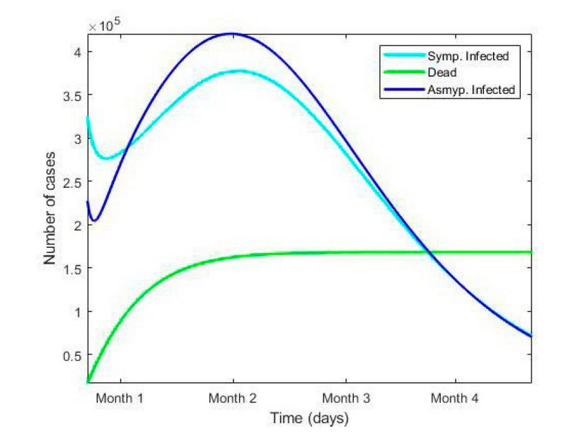
Figure 3. Dynamics of the infected symptomatic, asymptomatic infected and dead classes of the S-HI model in general community network in a 4-months period.

Figure 4. Dynamics of the infected symptomatic, asymptomatic infected and dead classes of the S-HI model in households network in a 4-months period.

Figure 5. Dynamics of the infected symptomatic, asymptomatic infected and dead classes of the S-HI model in workplaces network in a 4-months period.

Figure 6. Dynamics of the infected symptomatic, asymptomatic infected and dead classes of the S-HI model in agglomeration places network in a 4-months period.
In Figures 3 and 6, the three classes of interest present a similar dynamic. In community places such as neighborhoods, the contact between individuals is low because of the social distancing measures. This shows how the peak of infectious (infected and asymptomatic) individuals is relatively low. Also, the dead class stabilizes as the infected curve falls; this is accurate since only infected individuals can die. Here we consider agglomeration places as supermarkets where some ad-hoc rules were created to allow their operation. Although the contact weight in agglomeration places is slightly higher than in the general community, Figure 6 shows how the amount of infected, asymptomatic and dead individuals increases by 15% concerning Figure 3.

Table 1. Comparison of the increase in the number of Symptomatic Infected, Asymptomatic Infected and Dead individuals in each layer concerning the General Community.
.
The model shows that the curves reach their pick in every layer simultaneously. In Figures 5 and 4, the number of individuals in every class drastically increases by approximately 72% with respect to Figures 3 and 6. Notice that the household infected curve rises near 18% concerning the workplace curve. The contact weight in workplaces and households is higher because the dynamic within these networks of social distancing or the use of masks (only in households) does not intervene.
𝑹𝟎 Computation
As it's well known, for an infectious disease to be considered a pandemic, the reproduction number,
𝑅0, is greater than 1. To compute 𝑅0 we use the next-generation approach. Although we have 8 classes, we only consider the infected and infectious ones. Also, notice that at infection-free steady
𝐸 = 𝐴 = 𝐼 = 𝑄 = 0, then 𝑆 = 𝑁. Then we have the following linear system:

should discusses the results and how they can be interpreted from the perspective of previous studies and of the working hypotheses. The findings and their implications should be addressed in the broadest context possible. Future research directions may also be highlighted.

Table 2. Basic Reproduction Number, R_0, in 4 contact network layers: General community, Workplaces, Households and Agglomeration places.
The basic reproduction number for the general community, households, workplaces and agglom- operation places are 1.01, 1.68, 1.85, and 1.07, respectively, i.e., 𝑅0 > 1 for every layer, representing- ing an outbreak in each network. The expected number of cases directly generated by one infected case is higher when the individuals are in a closed space with no distancing measures, as in households. The contact rate is also high in workplaces such as offices, which is why the home office is so important. Here, agglomeration places are considered sites where all bio-security measures are fully complied with. Consequently, the reproduction number is relatively low. Finally, in the general community network, we have the lowest 𝑅0 because of the poor contact rate.
CONCLUSIONS
The whole world is being affected by the pandemic caused by the SARS-CoV-2 virus. Since the WHO declared it as such, it has been the subject of clinical and mathematical studies. In this work, we presented the S-HI model. This generalized SEIR model describes the dynamics of the SARS-CoV-2 virus in a community without herd immunity and performed simulations for 6 months.
The S-HI model consists of eight ordinary differential equations corresponding to susceptible individuals, exposed, asymptomatic infected, asymptomatic recovered, symptomatic infected, quarantined, recovered or dead. The parameters were taken as in7-9, and we took the cure and mortality rate as in.4
We studied the dynamics of the infected, asymptomatic and dead classes in 4 different networks: households, workplaces, agglomeration places and the general community. The dynamics of the three compartments have the same nature in each layer, as expected. It was observed how the speed of the disease considerably increased in the networks with the highest weight of contacts. This is because the probability of getting infected with the disease is quite high in closed spaces such as a home or workplaces. On the other hand, this speed is diminished in crowded places or ordinary squares thanks to social distancing and the use of masks. This is evidenced by the reproduction number, R0, which was greater than 1 in all networks, which is a necessary constraint for an infectious disease to be considered a pandemic.
Our results could not fit the data which underdeveloped governments have made public, mainly because of their lack of transparency. We must also note that we are not taking into account the disobedience in bio-safety issues by a segment of the population, nor are we taking into account the variants of the SARS-Cov-2 virus. This model only takes into account the original spread. Therefore, the S-HI model would fit, for example, the situation corresponding to the first wave of contagion after the mandatory lockdown.
Author Contributions: Conceptualization, Methodology, Resources, Supervision & Investigation, Paúl Me- dina-Vásquez; Methodology, Writing - Original Draft & Investigation, Ray Romero-Romero; Conceptualization, Methodology, Resources, Writing -Original Draft, Writing - Reviewing & Ediing, Supervision & Investigation, Juan Mayorga-Zambrano.
Funding: This research received no external funding. Institutional Review Board Statement: Not applicable. Informed Consent Statement: Not applicable.
Code Availability: https://drive.google.com/drive/folders/1THye0TIzjVMYoWtRObLNFjNXJ6Hld- nJP?usp=sharing
Acknowledgments: The authors thank the Yachay Tech community for its support during the whole Project.
Conflicts of Interest: The authors declare that they have no known competing financial interests or personal relationships that could have appeared to influence the work reported in this paper.
REFERENCES
1. D'Souza, G., Dowdy, D., Rethinking Herd Immunity and the Covid-19 Response End Game, Johns Hopkins University (2021). Re- trieved (9/21/2021) from https://publichealth.jhu.edu/.
2. Dietz, K., Heesterbeek, J.A.P., Daniel Bernoulli's epidemiological model revisited, Mathematical Biosciences 180 (2002) 1-21. https://doi.org/10.1016/S0025-5564(02)00122-0
3. Martcheva, M., An Introduction to Mathematical Epidemiology, Springer 2015. https://doi.org/10.1007/978-1-4899-7612-3
4. Peng, L., Wuyue, Y., Zhang, D., Zhuge, C., Hong, L., Epidemic analysis of COVID-19 in China by dynamical modeling, MedRxiv (2020). https://doi.org/10.1101/2020.02.16.20023465
5. Cuevas-Maraver, J., Kevrekidis, P.G., Chen, Q.Y., Kevrekidis, G.A., Villalobos-Daniel, V., Rapti, Z., Drossinos, Y., Lockdown Measures and their Impact on Single- and Two-age-structured Epidemic Model for the COVID-19 Outbreak in Mexico, Mathematical Biosciences 336 (2021). https://doi.org/10.1016/j.mbs.2021.108590
6. Liu, Q., Ajelli, M., Aleta, A., Merler, S., Moreno, Y., Vespignani, A., Measurability of the epidemic reproduction number in data-driven contact networks, PNAS USA 115 (2018) 12680-12685, 2018. https://doi.org/10.1073/pnas.1811115115.
7. Singhal, T., A Review of Coronavirus Disease-2019 (COVID-19), Indian J. Pediat. 87 (2020) 281-286. https://doi.org/10.1007/s12098- 020-03263-6. A model for the SARS-CoV-2 dynamics 11
8. Aragón-Nogales, R., Vargas-Almanza, I., Miranda-Novales, M., COVID-19 por SARS-CoV-2: la nueva emergencia de salud, Rev. Mex. de Pediatr´ıa 86 (2020) 213-218. https://dx.doi.org/10.35366/91871.
9. Di Gennaro, F., Pizzol, D., Marotta, C., Autunes, M., Racalbuto, V., Veronese, N., Smith, L., Coronavirus Diseasses (COVID-19) Current Status and Future Perspectives: A Narrative Review., Int. J. Environ. Res. Public Health 17 (2020) 2690. https://doi.org/10.3390/ijerph17082690
10. Cheynet, E., Generalized SEIR Epidemic Model (fitting and computation), Zenodo (2020). Retrieved from https://zenodo.org/rec- ord/3911854 https://doi.org/10.5281/zenodo.3911854
Received: December 23, 2022 / Accepted: January 30, 2023 / Published:15 February 2023
Citation: Medina-Vásquez P, Romero-Romero R, Mayorga-Zambrano J. A model for the SARS-CoV-2 dynamics in a population lacking herd immunity. Revis Bionatura 2023;8 (1)45. http://dx.doi.org/10.21931/RB/2023.08.01.45