2020.05.04.7
Files > Volume 5 > Vol 5 No 4 2020
INVESTIGATION / RESEARCH
Modeling of the spatial distribution of the vector Aedes Aegypti, transmitter of the Zika Virus in continental Ecuador by the application of GIS tools

Mario Bolivar Balseca Carrera1, Oswaldo Padilla Almeida2 and Theofilos Toulkeridis3
Available from: http://dx.doi.org/10.21931/RB/20120.05.04.7
ABSTRACT
In recent years Ecuador has suffered from the Zika virus. Geo-software and statistical software allowed the probabilistic identification of suitable ecological niche species, such as the vector Aedes aegypti, which is the leading cause of the Zika virus transmission, depending on the dependent and independent variables. These models require pre-weighted input, normalized, and rasterized inputs to continue the validation process to estimate their predictive performance through several statistics such as the confusion matrix or the Receiver Operating Characteristic Curve (ROC). It resulted that the Maxent method has been with the higher predictive performance with a value of Area Under Curve (AUC) = 0.998, which describes the areas of Zika with a greater probability of the transmission vector resembling the actual distribution of the species as a function of the presence data and the predictor variables. A large part of the Ecuadorian coastal territory yielded a statistical-based, probabilistic presence of the vector, being the most vulnerable before a possible epidemiological risk.
Keywords: Ecological niche model, GIS, Aedes Aegypti, Zika, Ecuador
INTRODUCTION
The vector Aedes aegypti is the leading cause of the Dengue, Chikungunya, and Zika viruses, transmitted by the bites of transmission of infected females1,2. In 1947, the virus was determined for the first time in Uganda, particularly in the forests of Zika3. It has been discovered in a Rhesus monkey during a study about the transmission of yellow fever in the jungle. In 2007, the first significant outbreak of Zika virus infection occurred in Yap Island (Micronesia), in which 185 suspected cases were reported4,5. Subsequently, an outbreak was recorded in French Polynesia, which began at the end of October 20136,7. There were around 10,000 cases where approximately 70 cases have been severe, with neurological complications (Guillain Barré syndrome, meningoencephalitis) or autoimmune (thrombocytic purpura, leukopenia). In 2014, cases were also recorded in New Caledonia and the Cook Islands8,9. In February 2014, the Chilean public health authorities confirmed a case of autochthonous transmission of Zika virus infection on Easter Island10. This appearance coincided with other transmission sources in islands of the Pacific, like French Polynesia, New Caledonia, and the Cook Islands. The Pan-American (PAHO) and World Health Organization (WHO), as well as the Network of Arbovirus Diagnostic Laboratories (RELDA) of the Americas, agreed on new guidelines to identify and confirm suspected cases of Zika in the affected countries. At the same time, the WHO and the scientific community seek to develop more precise tests11,12.
Vector diseases represent 17% of the estimated global burden of infectious diseases and, even in some cases, lethal13,14. In Ecuador, there is an endemic presence of the Aedes aegypti mosquito that has been closely related to climatic phenomena (temperature and humidity), causing direct and indirect economic losses that mainly affect the lower strata of society15-19. The Ministry of Public Health of Ecuador (MSP) has issued the mandatory epidemiological alert for health establishments of the Comprehensive Public Health Network and the Complementary Network, including all public and private establishments, which will allow the timely detection of all patients with suspicious symptoms, such as fever below 38.5°C, inflammation of the joints in hands and feet, red spots on the skin, conjunctivitis. Fever less than 38.5°C and the possible presence of conjunctivitis differentiate Zika fever symptoms from the symptoms of dengue and chikungunya15. Therefore, the National System of Vigilance and Early Warning for the control of the vector of dengue and yellow fever has proposed a project that proposes obtaining climatological, socio-economic, and biological information of the Aedes aegypti mosquito to deploy it with Geographic Information Systems (GIS) to develop an Early Warning System for the Control of the Vector of Dengue and Yellow Fever, developing predictive mathematical models for dengue based on the relationship between entomological, epidemiological, socio-economic and climatological data15.
These models generate predictions regarding the species' distribution and environmental requirements, enable the identification of the variables that best predict favorable habitats, allow ecological testing hypotheses about the distribution of organisms, and evaluate the impacts of possible environmental changes. This type of ecological distribution modeling (Maximum Entropy, Logistic Regression, etc.) has been used in the current study to identify suitable areas for the development and proliferation of Aedes aegypti, the transmitter of the parasite that causes the Zika virus20.
METHODOLOGY
Methods for Ecological Niche Modeling
Currently, there is a wide variety of methodologies to perform ecological niche modeling by using mathematical algorithms and automatic learning methods that require biological data of the species and the application of environmental variables21-26. Mainly these methodologies are based on three statistical classification techniques, namely discriminant, descriptive, and mixed. In the discriminant techniques, the species' biological data are needed being presence and absence to build the statistic. Among them are classification trees (CART), artificial neural networks (AN), generalized linear models (GLMs), generalized additive models (GAMs), maximum entropy models (MAXENT), multivariate adaptive regression splines (MARS) among several others27-32. Descriptive techniques require biological data of the species with presence only. Examples of such techniques include BIOCLIM, BIOMAP, and Ecological Niche Factor Analysis-Biomapper (ENFA), among others33-36. Mixed techniques use both descriptive and discriminating techniques, making their pseudo-absences. Among them are Desktop-GARP and OM-GARP, among others37-39.
In some cases, the algorithms have been implemented in a friendly way for the user through software packages that allow describing the relationship between the environment and the species, which are generally available for free to later integrate it into a GIS to obtain cartographic products40.
Information collection
To model the spatial distribution of a species, it has been necessary to have two types of information: the dependent variables (presence, absence, or pseudo-absence data) and independent variables (predictors). Furthermore, we needed a series of ecological modeling techniques that have been used, such as Maxent, MARS, SPSS, that emulate or demonstrate the research result through statistical modeling, thus determining the suitability of the habitat for the development of the species. The ArcGis version 9.x software has also been used to collect, organize, manage, generate, and analyze the necessary supplies for each model used. As generated, all the collected information has been handled with the WGS84 Reference System with UTM projection, zone 17 South.
a) Dependent Variables
The records of the presence of the vector Aedes aegypti have been obtained from periodical publications (Gazettes) issued by the Ecuadorian Undersecretary of Public Health Surveillance through the National Directorate of Epidemiological Surveillance specialized in Diseases Transmitted by Vectors, which since the end of 2015 (weeks epidemiological studies 52-53) began to publish them. The data for modeling the species' distribution has been taken until the report issued on September 14, 2016 (epidemiological weeks 1-36).
As the vector usually transmits the Zika virus, Aedes aegypti, therefore, only the localities where there are confirmed autochthonous cases of the virus have been georeferenced (42 records), which according to the WHO, are local epidemiological contagion records11, meaning that there is the presence of the vector in situ. Table 1 and Figure 1 summarize the provinces with their respective cantons, where the confirmed autochthonous and imported cases of Zika Virus (ZikaV) have been encountered in continental Ecuador.
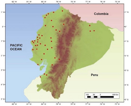
Figure.1: Presence of the Vector Aedes aegypti in continental Ecuador41.
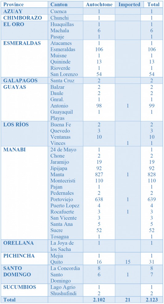
Table 1: Confirmed cases of autochthonous and imported Zika Virus41.
Data of absence or pseudo-absence of Aedes aegypti
The data of absence are fundamental in the species' distribution models; however, currently, there are no scientific investigations that determine areas not suitable for the reproduction of the vector because it adapts easily to any environment. Therefore, pseudo-absences have been created that are absences estimated from the vector's biological, ecological, and historical data. The pseudo-absences for the present study have been generated based on the presence data as suggested by several authors, who state that from them, a radius of 30 km has been established in which the environmental, topographic, and landscape conditions stabilize, that is, there is a probability of the presence of the vector within this area. This delimitation has been conducted with the ArcGis buffer tool. Later these areas have been erased from our study area (mainland Ecuador) using the ArcGis erase tool to finally create random points that exceed the total sample of the presence of the vector (48 pseudo-absence points) using the create random points tool from ArcGis (Figure.2).
The pseudo absence is generated by taking the same number of points plus an additional 10% in a random form with a minimum distance of 30 km between points since this seeks to ensure that the environmental and physical conditions are not the same, then the points are discarded that are less than 30 km (again) from the points of presence.
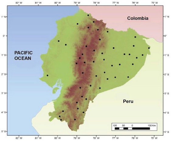
Figure.2: Pseudo-absence of the Vector Aedes aegypti in the mainland of Ecuador
b) Independent Variables
The 19 iboclimatic variables have been taken from the Worldclim Website (http://www.worldclim.org/), which brings together a set of global climate data with a 30-second spatial resolution that is approximately 1km² on the Equator line. This portal's offered layers have been created by interpolating the averages of monthly, quarterly, and annual climatic data for each station. The variables that have been included in the model are average annual temperature, an average of the day range, isothermality, seasonal temperature, maximum temperature of the hottest month, minimum temperature of the coldest month, annual temperature range, the average temperature of the wettest quarter, average temperature of the driest quarter, average temperature of the warmest quarter, average of the coldest quarter temperature, annual precipitation, precipitation of the wettest month, precipitation of the driest month, seasonal precipitation (Coefficient of variation), precipitation for the quarter wettest, precipitation of the driest quarter, precipitation of the hottest quarter and precipitation of the coldest quarter.
The layers are worldwide in .grid format; therefore, all the used variables have been cut to the size of the study area (Ecuadorian mainland) with the same pixel size (1000x1000) meters and in the same way, the same number of rows and columns (650x721) with the ArcGis "Extract by Mask" tool (Figure.3a-e).
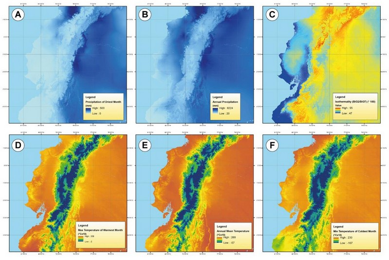
Figure.3: Examples of the bioclimatic variables for modeling the Aedes aegypti in the Ecuadorian mainland, as taken from the Worldclim Website (see text). A) precipitation of the driest month; B) annual rainfall; C) isothermality: D) maximum temperature of the warmest month; E) central annual temperature; F) minimum temperature of the coldest month
Geographic Variables
The geographical variables that have been used to perform the modeling have been part of the base cartography with a scale of 1: 50000, which has been included in the Geoportal of the National Information System SNI (http://sni.gob.ec/inicio), except for the altitude. We realized a previous process to each variable, is described below, before becoming part of each model.
a) Altitude
The information corresponding to the altitude has been compiled from the Worldclim Web Site, which relied on the Topographic Radar Shuttle Mission (SRTM) driven by the NASA. At this moment, a digital model of the Earth's surface has been developed based on the information collected from space. Like the environmental variables, the resolution and the size of the pixel have been cut and adjusted to the study area with the ArcGIS Extract by Mask tool.
b) Areas susceptible to flooding
The raw information of this variable has been in vector format, therefore the ArcGis "Euclidean distance" tool has been used, which, when rasterized, provided the distance from each cell to the nearest source of the areas susceptible to flooding (Figure.4b).
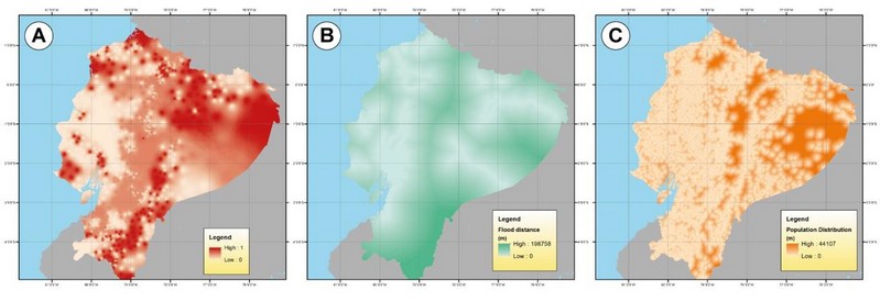
Figure.4a-c. Modeling of Aedes aegypti with different variables: A) Poverty Index; B) Flood distances C) Populated Centers.
c) Populated centers
Like the previous variable, the raw information has been treated in the identical form and followed the same procedure (Figure.4c).
d) Land use
For the land-use variable, Saaty's Analytical method has been used, which has been based on hierarchizing the components or variables by means of numerical values for the preference judgments, thus determining which variable has the highest priority42,43. In table 2, the land use at the national level has been weighted according to the percentage of presences (Figure.5) and the characteristics that result in them more apt to become the vector's habitat. Later the information has been rasterized using the tool ArcGis "Feature to Raster" based on a new field called "weights" where the range of values has been between 0 and 1 (Figure.6).
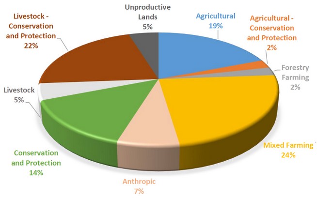
Figure.5: Presence of Aedes aegypti in the function of Land use
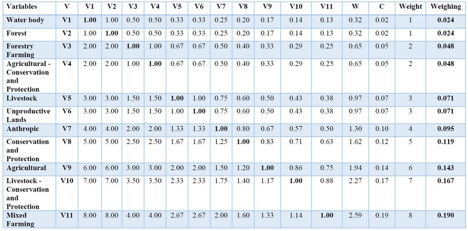
Table 2. Matrix of Saaty about the land use42,43.
Socio-economic variables
As stated above, the variable about the Poverty Index has been linked to the quality of life in the socio-economic environment. That is, if the quality of life has been low, there will be houses without access to potable water through a water network, in addition to not having drainage systems, so the population is forced to store water in internal or external tanks, which favors the proliferation of the Aedes aegypti vector. In the Geoportal of the National Institute of Statistics and Censuses (http://www.ecuadorencifras.gob.ec/geoportal/) this information has been in vector format has been rasterized using the ArcGis "IDW" interpolation tool. This process calculated each of the cells' values through a linearly weighted combination based on a given field. In the present study, the percentage of the poverty index through the centroids of all the parishes nationwide has been considered as illustrated in Figure 4a. The same has been done about the flood distances and the populated centers (Figure.4b and Figure.4c). Hereby, it is about the variables taken in the model, being predictor variables. The summary of the predictor variables that have been used for the Aedes aegypti vector modeling has been listed in Table 3.
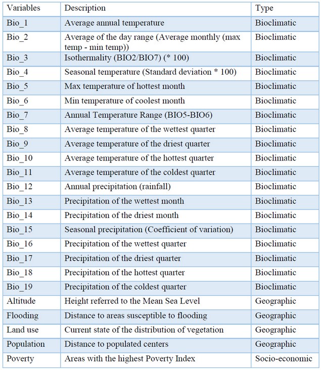
Table 3: Predictor variables for the modeling of Aedes aegypti
Not all of the above-described variables contributed in the same way to each model, which includes that even dispense with any of them has been possible due to the statistic performed by each modeling method.
Normalization of the variables
Most distribution models of species require the homologation of the values of both dependent and independent variables; therefore, the information has been dimensioned and referenced within the same scale. That is, in a range of [0,1] where it has been considered that there has been a greater probability of the presence of the vector when the values have been closer to "1". Within the study area, the maximum and minimum values have been determined with the presence of the vector of each one of the variables, using the ArcGis "Extract Multi Values to Points" tool, with which the extreme conditions for vector survival have been able to be established and in turn excluding the zones with the absence of it, as evidenced in Table 4. Using the ArcGis "Reclassify" tool, the excluded ranges of the raster that has the data of the particular variable have been assigned to a value of "0".
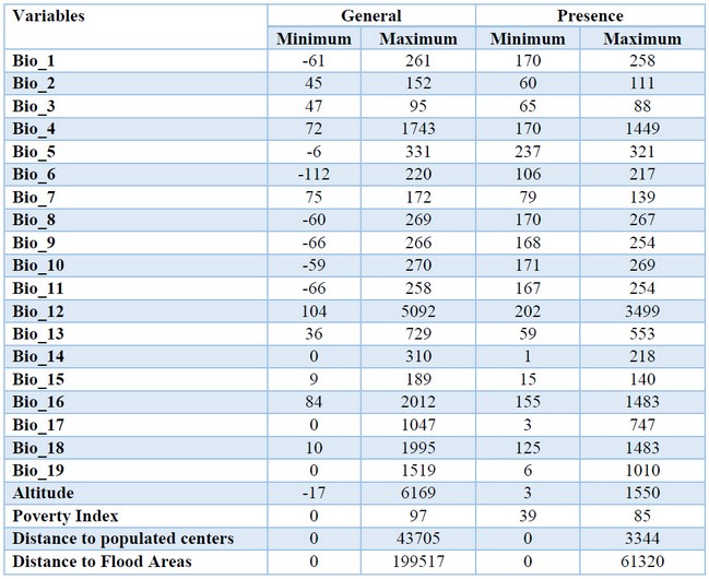
Table 4: Maximum and minimum values of the Independent Variables
Once the maximum and minimum values with the presence of a vector have been obtained, the formula (1) to normalize has been used for each of the variables:
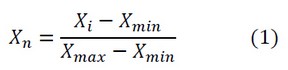
Where Xn is the normalized variable, Xi is the variable, Xmin and Xmax represent the minimum and maximum values, respectively. The land-use variable did not perform this process because it has been previously normalized by applying the Saaty method42,43.
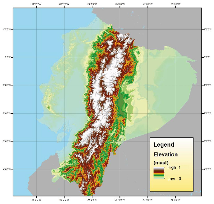
Figure.6: Reclassification of Variable values
Distribution Models of the species
In the current study, several statistical models have been applied to determine which of them is the most optimal to predict the spatial distribution of the Aedes aegypti mosquito vector of the Zika virus. The used models have been Maxent, ROC Curve Analysis, Fuzzy Logic, Logistic Regression, and Multivariate Adaptive Regression Splines (MARS).
a) Maxent (Maximum Entropy)
For the application of maximum entropy model or Maxent, free software with the same name MaxEnt has been used31. This statistic is discriminant and requires presence and absence data. However, Maxent provides its absences, called "background". Additionally, this virtual platform does not require that the predictor variables be normalized because this statistical process is carried out internally by the program. Maxent is a software used to calculate geographic distribution models, in which the relationship of the presence data of a species and different predictive spatial variables are analyzed. The model itself can be spatialized and can represent the probability of the localization of the species.
b) Receiver Operating Characteristic analysis (ROC)
The ROC curve (Receiver Operating Characteristic analysis), is a statistic that graphically represents the discriminative capacity of any model for all its possible cut points. It needs the data to be evaluated to be of presence/absence to define the threshold or criteria necessary for predicting the species44. The ROC curve is obtained by relating the sensitivity that is the fraction of true positives (y-axis), with the "1- specificity" which is the fraction of false positives (x-axis), for ease of calculation is used the expression "1- specificity" so that sensitivity and specificity vary in the same direction when the threshold is defined45.
The derived statistic is the area under the ROC curve, or Area Under Curve (AUC), which provides a full measure of the predictive capacity as well as assessing the best fit in ecological niche models, defined by 45 as:
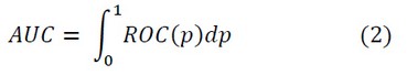
The AUC is calculated by adding the area under the ROC curve and takes values from 0 to 1, where values less than 0.5 indicate that the model is naughty since it classifies erroneously more cases than chance. AUC values of 0.5 to 0.7 are considered a low performance of the model, while values between 0.7 to 0.9 presume a moderate model's moderate performance. Values greater than 0.9 estimates a high level of the model, indicating that all cases have been classified correctly46. The AUC values are not affected by changes in the prevalence of the species, and therefore it is a reliable statistic in the comparison of models. Some studies have demonstrated that AUC does not decrease with increasing species prevalence47. Among the advantages that the AUC calculation provides is the possibility of comparing several methods, whatever the type of output values, because it only needs the distributions of these values48.
c) Diffuse Logic or Fuzzy Logic
The main application of Fuzzy Logic is to represent quantitative values (numerical values between 0 and 1) through qualitative linguistic inputs, employing managing domains that are not within the scope of classical logic49. For Fuzzy Logic, the functions that are applied are the Sine and the Cosine because the range in which one works is between 0 and 1. The methodology that fuzzy Logic manages consists of determining the interaction of each variable that is part of the model with the probability of the presence of the species within three possible scenarios or cases. We analyzed how the predictor variables react with respect to the probability of the presence of the species to determine which of the cases raised in the Fuzzy methodology will be applied (table 5).
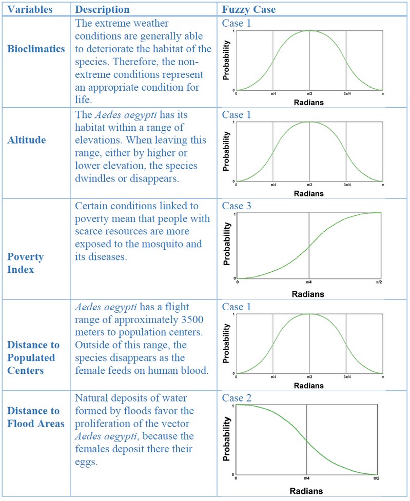
Table 5: Analisis of the variables
For the land-use variable, it has not been necessary to determine Fuzzy's corresponding case because previously, this process was performed using the Saaty method.
Once the normalization process has been applied and the corresponding scenarios (cases) of the fuzzy Logic have been identified, the value of the variables has been transformed to radians using the following formula:
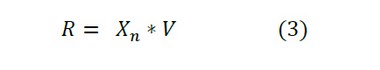
Where R is the value of the variable in radians, Xn is the normalized variable and V is the value of “p”or “p/2” according to the range corresponding to each scenario.
In order to analyze the probability of occurrence of each variable it has been necessary to use the following equation:
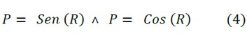
The trigonometric functions that have been used were the sine and the cosine because after performing the analysis of scenarios proposed by Fuzzy, it has been determined that the model has all three cases.
Finally, we averaged the probabilities of all the variables using the ArcGis "Raster Calculator" tool by applying the equation described below:
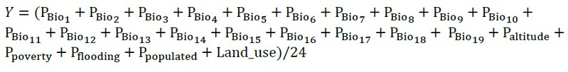
Where Y is the probability of the model.
d) Logistic regression
For the application of the Logistic Regression method, we used a statistical software called Statistical Package for Social Sciences (SPSS), which is very often used to perform analytical processes to conduct research and make better decisions. Within this statistical package, the element of binary logistic regression is necessary to calculate the constant and the coefficients that best fit the functional expression of the variables. The logistic regression method is discriminant; therefore, it is necessary to have the needed inputs such as predictor variables, presence, and pseudo-absence data that have been previously generated.
To perform the corresponding statistical analyzes in the SPSS 23 program, it is necessary to generate a matrix with all the predictor variables' values already normalized according to the points of absence and presence. This information has been obtained through the ArcGis "Extract Multi Values to Points" tool. The type of regression that has been chosen for the current study has been binary logistic, because the values of the inputs are dichotomous, being within the range [0,1] which are optimally fitting this statistic to the model. Afterward, we configured which are the dependent and independent variables (covariables).
Several statistics have been obtained from the execution of the program that evaluates the reliability of the results, such as classification tables for the variables, omnibus tests, correlation matrix and, mainly, the coefficient table needed to generate the model (β0, β1, β2…. β p) , as indicated in Figure.7.
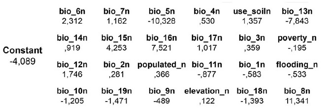
Figure.7. Example of a table with coefficients of the variables
In this way, the values of the constants have been multiplied by each variable with the help of the ArcGis "Raster Calculator" tool, following the formula of the logistic regression:

Where Y is the probability of the model.
e) Multivariate Adaptive Regression Splines (MARS)
The MARS program with other statistical products such as classification and regression tree (CART), TreeNet, and Random Forests, are all focused on elaborating predictive and descriptive models to analyze databases of any size and of different complexity 32,50-51. The MARS method proposes a complete analysis of the variables according to the importance of each of them for the prediction of the event, adjusting the model not only to a predictive curve but rather dividing it into zones (base functions) through nodes or the so-called inflection points, which improves the results. Like the previous models, the inputs needed to apply the model are the predictor variables, presence, and pseudo-absence data.
MARS generates an internal process of iterations called "forward" on the original predictor variables' base functions. Subsequently, the program will discard those that least fit the model through another process called "backward", which converts the original variable X into a new variable defined as: max (0, X-c) or max (c-X), where c is the threshold established by the nodes, as shown below.
BF2 = max( 0, 0.416 - [bio_15n])
BF3 = max( 0, [flooding _n] - 0.015118)
BF4 = max( 0, 0.015118 - [flooding_n])
BF5 = max( 0, [poverty_n] - 0.723404)
BF6 = max( 0, 0.723404 - [pobreza_n])
BF7 = max( 0, [populated_n] - 0.392163)
BF8 = max( 0, 0.392163 - [populated _n])
BF9 = max( 0, [bio_8n] + 5.96046e-008)
BF11 = max( 0, 0.72619 - [bio_5n])
BF12 = max( 0, [bio_12n] - 0.863209)
BF14 = max( 0, [bio_2n] - 0.764706)
Finally, MARS creates a final predictive equation that is defined by the generated base functions, which in turn are multiplied by the coefficients that best fit the model, by using the ArcGis "Raster Calculator" tool.
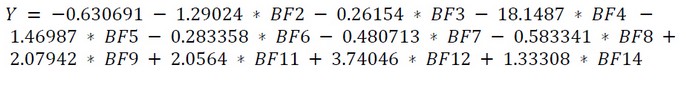
Where Y is the probability of the model.
Standard Deviation and Adjustment of Models
The standard deviation is a set of data or a measure of dispersion that indicates how far the obtained values may be moved away from the average. That means that this statistic's importance is based on the probability that an event will occur or not. The values of the standard deviations of the models applied have been described in Table 6 in addition to their maximum, minimum, and arithmetic mean values.
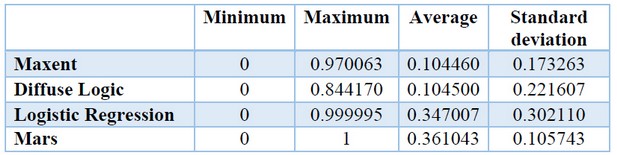
Table 6: Standard Deviation of Models
The adjustment has been conducted on the previously normalized final models within a range of [0,1], depending on the standard deviation, applying the following equation:
N = Measured Value – Calculated Value (4)
Where N is the adjustment value, the Measured Value is the maximum value at which the models could arrive, that is to say, "1" (probability of presence), and the Calculated Value is the value of the standard deviation of the averages of probabilities of the different models.
Table 7 lists the standard deviations of the models and the adjustment made to each of them.
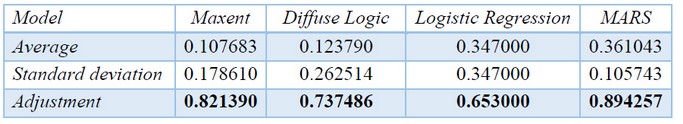
Table 7: Adjustment of the Models
RESULTS
To select the model with a more excellent predictive performance of the spatial distribution of the vector Aedes aegypti within the Ecuadorian mainland, several analyzes and comparisons have been performed, both statistics and graphs of the four applied models.
a) Analysis of the adjustment of the models
By analyzing the adjustment of the previously normalized models (Table 8), it has been observed that the MARS method with an adjustment of 0.894 has been the closest to the value of one, demonstrating a low dispersion of its data concerning the mean, which means that the prediction has been significant. Next are the methods of Maxent and Fuzzy Logic with adjusted values within an acceptable range of 0.821 and 0.737, respectively. Finally, the logistic regression method with the adjusted value of 0.653, describes a low predictive performance.
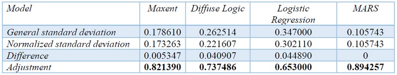
Table 8: Analysis of the Adjustment of the Models
b) Analysis of the AUC Curve of the models
The predictive capacity of the models has been validated by the AUC statistical analysis from the ROC curve, whose main function has been to calculate the sensitivity and specificity of the values of the occurrences of the species by intersecting the presences with the layers (raster) of each of the obtained models. The ROC curve has been based on the union of different cutting points, corresponding on the Y-axis to the "sensitivity" and the X-axis to the "1-specificity". The two axes contain values between 0 and 1 (0% to 100%), while the confidence interval that has been used for the analysis has been of about 95%.
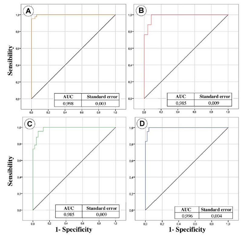
Figure.8: Analysis of the ROC Curve, a) Model Maxent; b) Fuzzy Logic Model; c) Logistic Regression Model; d) MARS model (4.1-4.4)
The graphs of the ROC curves have been superimposed in Figure 9, illustrating satisfactory predictive results> 0.9 of the AUC in all models, which means that within the confusion matrix environment, there have been predictions with authentic presences and true absences. However, the model that has been closest to "1" is the Maxent Model (Figure.8a) with a value of AUC = 0.998. Then the MARS Model (Figure.8d) with a value of AUC = 0.996 and finally with a similar value the models of Fuzzy Logic (Figure.8b) and Logistic Regression (Figure.8c) of AUC = 0.986.
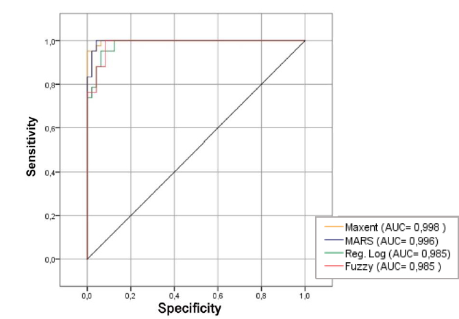
Figure.9: Analysis of the ROC Curve of all four models
c) Graphic Analysis of the models
As a result of the comparison of the used models for the prediction of the spatial distribution of the Aedes aegypti vector, it has been evidenced that both the Maxent models (Figure.10a) and the Fuzzy Logic models (Figure.10b) conform to the real distribution of the vector because the areas most likely predicted by these models have been close to the points of presence. Additionally, these zones must meet the zones with biological parameters essential for the survival of the vector such as low altitudes, being not higher than 1600 meters above sea level, and distances to population centers that do not exceed 4000 meters since the females need to have enough blood as a source of proteins to multiply for the production of their eggs. The models of Logistic Regression (Figure.10c) and MARS (Figure.10d) predict a high probability of the vector's presence in almost the entire coastal region without discriminating zones where absences may exist due to climatic, topographic, and other factors.
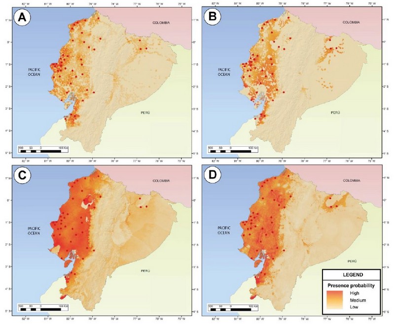
Figure.10: Distribution of Aedes aegypti: A) Model Maxent; B) Fuzzy Logic Model; C) Logistic Regression Model; D) MARS model
d) Logistic Regression Model
After having performed several analyzes and comparisons, both statistics and graphs of the four applied models in the present investigation, we concluded that the Maxent model has a better predictive performance of the spatial distribution of the vector Aedes aegypti, since it represents a satisfactory performance in the analysis of ROC curve, with a value AUC = 0.998, and with an adjustment of the standard deviation 0.821390 (Table 8), only below the MARS model. In addition, it visually describes the areas with the most significant probability of the vector, which conveniently resembles reality according to the present data and the predictor variables.
DISCUSSION
Methods used
Maxent has been established as the model with the highest predictive performance after several statistical validations. Besides, it visually describes the zones with the highest probability of the vector's presence, which also resembles the vector's real distribution according to the present data and the predictor variables. The Fuzzy or Fuzzy Logic methodology determines quite good predictions with a predictive performance scarcely inferior to the Maxent method, which constructs its model based on the generation of background due to the necessity that its algorithm requires, sometimes causing an over the adjustment of the model. Unlike Fuzzy, which makes its predictions based on the predictor variables, presence, pseudo-absence data, and improvement if the model will include absence data sampled in the field. The logistic regression methods and MARS registered good values in the statistical analyzes. However, graphically they register a high probability of the vector in almost all the coastal regions without discriminating zones in which there could be absences of the same due to climatic, topographic factors, among others.
Delimitation of suitable zones for the presence of the vector
The estimation of the areas with the highest probability of the presence of the Aedes aegypti vector has been determined by analyzing their frequency within the study area, resulting in the histogram of Figure 11. It illustrates that the lowest number of frequencies is in a range of (0-30%) with only 4 presences, an intermediate frequency with a value of 18 presences in a range of (30-60%) and half of the presence data with a value of 22 in the range of (60-100%).
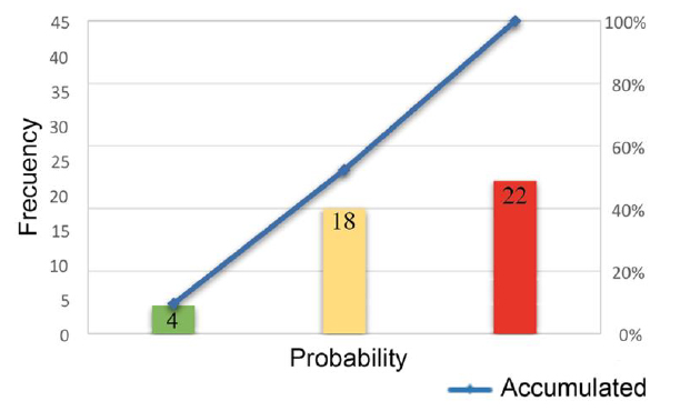
Figure.11: Probability Histogram
Figure 12 graphically illustrates the range of probabilities that have been previously determined, which clearly shows that the coastal region is the most suitable for the vector's existence.
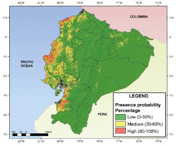
Figure.12. Probabilities of the presence of the vector Aedes aegypti
According to the frequency analysis of the vector within the study area that has been previously performed, it has been estimated that the zones with the highest probability of the presence of the vector are within the range (60-100%) that is proportional to the epidemiological risk. Subsequently, only areas with a high probability of the presence of the vector have been reclassified, as documented in Figure 13.
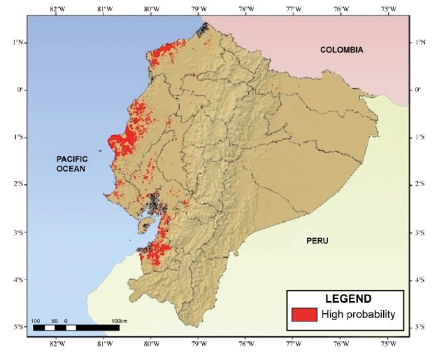
Figure.13: Suitable areas for the presence of vector Aedes aegypti
The ideal zones for the Aedes aegypti vector's presence cover an area of 7806 km2, representing 3.15% of the territory of the Ecuadorian mainland. This area is divided into 16 provinces (111 cantons). There is a high presence in the coastal region in important localities such as Guayaquil, Machala, Babahoyo, Portoviejo, Salinas, and others, a low presence in the Amazon region and absence entirely in the Highlands region (Table 9).
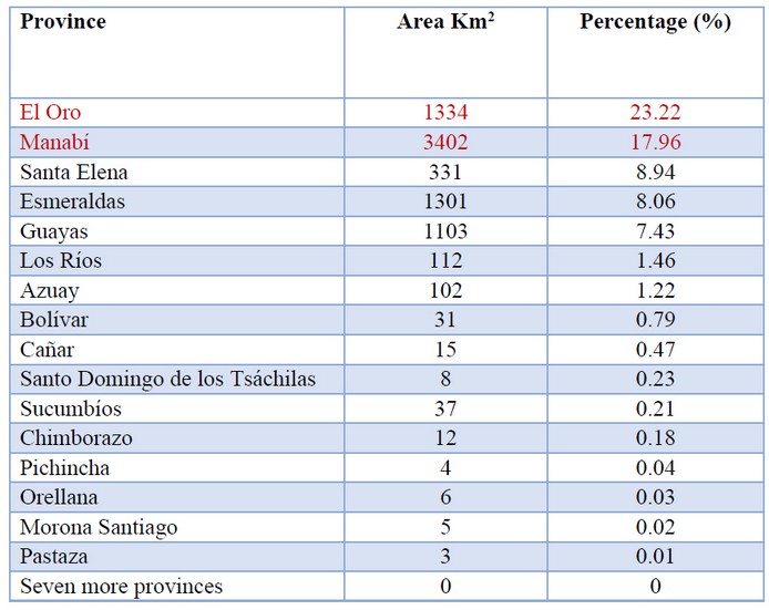
Table 9: Provinces with higher epidemiological risk
Characterization of the areas with the highest epidemiological risk
There are several zones along the Ecuadorian coast that have been suitable for the characterization of epidemiological risk, as the probability of the vector's presence is very high. However, the provinces of Manabí and El Oro have been considered for this study because more than 15% of their territorial areas have been exposed to a vector's possible spatial distribution. The province of Manabí has 22 cantons, of which 21 determine a possible presence of the vector, while the province of El Oro has a territorial expansion on a smaller scale compared to Manabí, with 14 cantons of which all show the presence of the vector.
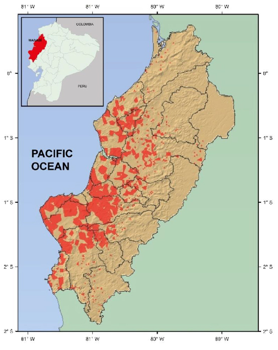
Figure.14: Manabí province with suitable areas for the presence of vector Aedes aegypti
The province of Manabi has about 18,400 km², about 1.369.780 inhabitants, with a poverty rate of about 39.8%. The precipitation has a range of 500 to 1000 mm per year, an average temperature of 25°C, and a dry subtropical climate to tropical humid. Manabí has approximately 350 km of maritime coastline, with important geographical and climate features52. Certain areas of the province are predisposed to flooding in the winter seasons with higher rainfall53,54. There is a predominance of 51.3% cultivated pastures representing little more than half of the used provincial area. The mountains and forests with 21.5% and the permanent crops with 13.2% added to the grassland areas document the existence of protected areas and areas suitable for livestock55. The most extensive parts of the province have high deficit rates in essential residential services (water, wastewater disposal, electricity supply) with 80% and 61.20%, respectively54.
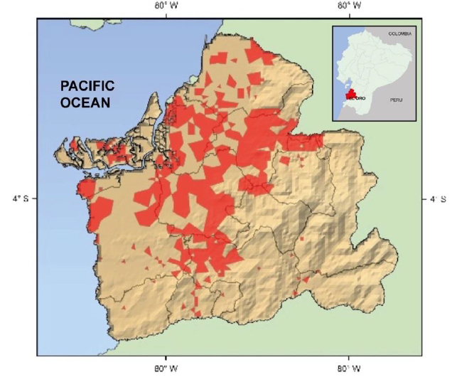
Figure.15: El Oro province with suitable areas for the presence of vector Aedes aegypti
The province of El Oro, has an area of about 5767 km², about 648,316 inhabitants with a poverty rate of about 23.4%. The precipitation has a range of 200 to 1500 mm per year, an average temperature of 25°C and a dry coastal climate, tropical Savanna, and rainy winters. This province is divided into two areas, to the northwest, the foothills that descend to the Gulf of Guayaquil are the plains, where banana is grown, and the southeast mountainous area that is crossed by the Western Cordillera of the Andes, where the temperature decreases according to the height54. The area of land occupied by agricultural activity is 457,025 ha, distributed as follows: 2.17% of transitory crops; 53.56% pastures (cultivable and natural); 12.36% forests; 13.45% other uses, rest and páramos55. Some 79% of the total population of the province is concentrated in the urban area, while the residual 21% remain in the rural area54.
Both provinces have a significant environmental and social problem where pollution and high demographic and poverty rates are the most representative.
CONCLUSIONS
Maxent has been established as the model with the highest predictive performance after several statistical validations. In addition, it visually describes the zones with the highest probability of the presence of the vector, which additionally resembles the real distribution of the vector according to the present data and the predictor variables.
The Fuzzy or Fuzzy Logic methodology determines good predictions with a predictive performance scarcely inferior to the Maxent method, which constructs its model based on the generation of background due to the necessity that its algorithm requires, sometimes causing an over the adjustment of the model. Unlike Fuzzy, which makes its predictions based on the predictor variables, presence, pseudo-absence data, and improvement, the model will include absence data sampled in the field.
The logistic regression methods and MARS registered good values in the statistical analyzes. However, graphically they register a high probability of the vector in almost all the coastal regions without discriminating zones in which there could be absences of the same due to climatic, topographic factors, among others.
The areas with the highest probability of the vector Aedes aegypti generally cover an area of 7806 km2 distributed in 16 provinces, located almost exclusively in the coastal region. There, the provinces of Manabí and El Oro, due to their geographical, climatic, and even socio-economic characteristics, such as altitude, temperature, precipitation, and environments, associated with human life conditions, establish favorable sites with a greater probability of the presence of the Aedes aegypti vector.
The spatial distribution model of the Aedes Aegypti allowed the characterization of the zones with a greater probability of the presence of the vector. This way, we have been able to define the ecological dynamics of transmission of ZIKA, the evaluation of the epidemiological-economic impact, and the intervention strategies that should be taken before a possible epidemiological risk in Ecuador.
REFERENCES
1. Foy, B. D., Kobylinski, K. C., Foy, J. L. C., Blitvich, B. J., da Rosa, A. T., Haddow, A. D., Lanciotti, R.S. and Tesh, R. B. (2011). Probable non–vector-borne transmission of Zika virus, Colorado, USA. Emerging infectious diseases, 17(5), 880.
2. Ioos, S., Mallet, H. P., Goffart, I. L., Gauthier, V., Cardoso, T., & Herida, M. (2014). Current Zika virus epidemiology and recent epidemics. Medecine et maladies infectieuses, 44(7), 302-307.
3. Dick GW, Kitchen SF, Haddow AJ (1952) Zika virus. I. Isolations and serological specificity. Trans R Soc Trop Med Hyg 46: 509-520.
4. Lanciotti, R. S., Kosoy, O. L., Laven, J. J., Velez, J. O., Lambert, A. J., Johnson, A. J., Stanfield, S.M. & Duffy, M. R. (2008). Genetic and serologic properties of Zika virus associated with an epidemic, Yap State, Micronesia, 2007. Emerging infectious diseases, 14(8), 1232.
5. Duffy, M. R., Chen, T. H., Hancock, W. T., Powers, A. M., Kool, J. L., Lanciotti, R. S., Pretrick, M., Marfel, M., Holzbauer, S., Dubray, C. and Guillaumot, L. (2009). Zika virus outbreak on Yap Island, federated states of Micronesia. New England Journal of Medicine, 360(24), 2536-2543.
6. Cao-Lormeau, V. M., Roche, C., Teissier, A., Robin, E., Berry, A. L., Mallet, H. P., Sall, A.A. and Musso, D. (2014). Zika virus, French polynesia, South pacific, 2013. Emerging infectious diseases, 20(6), 1085.
7. Cauchemez, S., Besnard, M., Bompard, P., Dub, T., Guillemette-Artur, P., Eyrolle-Guignot, D., Salje, H., Van Kerkhove, M.D., Abadie, V., Garel, C. and Fontanet, A. (2016). Association between Zika virus and microcephaly in French Polynesia, 2013–15: a retrospective study. The Lancet, 387(10033), 2125-2132.
8. Musso, D., Nilles, E. J., & Cao‐Lormeau, V. M. (2014). Rapid spread of emerging Zika virus in the Pacific area. Clinical Microbiology and Infection, 20(10).
9. Dupont-Rouzeyrol, M., O'Connor, O., Calvez, E., Daures, M., John, M., Grangeon, J. P., & Gourinat, A. C. (2015). Co-infection with Zika and dengue viruses in 2 patients, New Caledonia, 2014. Emerging infectious diseases, 21(2), 381.
10. Tognarelli, J., Ulloa, S., Villagra, E., Lagos, J., Aguayo, C., Fasce, R., Parra, B., Mora, J., Becerra, N., Lagos, N. and Vera, L. (2016). A report on the outbreak of Zika virus on Easter Island, South Pacific, 2014. Archives of virology, 161(3), 665-668.
11. WHO (World Health Organization), (2016a). Zika virus research agenda. Geneva, Switzerland: 19pp
12. WHO (World Health Organization), (2016b). Zika situation report: neurological syndrome and congenital anomalies. Geneva, Switzerland: 6pp
13. Bhatt, S., Gething, P. W., Brady, O. J., Messina, J. P., Farlow, A. W., Moyes, C. L., Drake, J.M., Brownstein, J.S., Hoen, A.G., Sankoh, O. and Myers, M. F. (2013). The global distribution and burden of dengue. Nature, 496(7446), 504.
14. Hotez, P. J., Alvarado, M., Basáñez, M. G., Bolliger, I., Bourne, R., Boussinesq, M., Brooker, S.J., Brown, A.S., Buckle, G., Budke, C.M. and Carabin, H. (2014). The global burden of disease study 2010: interpretation and implications for the neglected tropical diseases. PLoS neglected tropical diseases, 8(7), e2865.
15. MSP (Ministerio de Salud Pública del Ecuador), (2015). Alerta Epidemiológica: Ante La Posibilidad De Introducción Del Virus Zika En Ecuador. Quito: Ministerio de Salud Pública. http://www.salud.gob.ec/boletin-de-prensa-alerta-epidemiologica-ante-la-posibilidad-de-introduccion-del-virus-zika-en-ecuador/
16. Zambrano, H., Waggoner, J. J., Almeida, C., Rivera, L., Benjamin, J. Q., & Pinsky, B. A. (2016). Zika virus and chikungunya virus coinfections: a series of three cases from a single center in Ecuador. The American journal of tropical medicine and hygiene, 95(4), 894-896.
17. Padilla, O., Rosas, P., Moreno, W., & Toulkeridis, T. (2017). Modeling of the ecological niches of the anopheles spp in Ecuador by the use of geo-informatic tools. Spatial and spatio-temporal epidemiology, 21, 1-11.
18. Perugachy Kindler, J.T., Zapata, J., Ordoñez, E., Toulkeridis, T. and Zapata A. (2020). Ecological Niche Modeling of Vector Species of the American Trypanosomiasis Disease (Chagas), in Continental Ecuador. 7th International Conference on eDemocracy and eGovernment, ICEDEG 2020, 165-174.
19. Toulkeridis, T., Tamayo, E., Simón-Baile, D., Merizalde-Mora, M.J., Reyes –Yunga, D.F., Viera-Torres, M. and Heredia, M. (2020). Climate change according to Ecuadorian academics–Perceptions versus facts. La Granja, 31(1), 21-49
20. Rotela. (2014). Epidemiologìa panorámica: introducción al uso de herramientas geoespaciales aplicadas a la salud pública. Ciudad Autónoma de Buenos Aires: Comisión Nacional de Actividades Espaciales; Ministerio de Planificación Federal Inversión Pública y Servicios Ministerio de Salud de la Nación. 110pp
21. Soberón, J., & Nakamura, M. (2009). Niches and distributional areas: concepts, methods, and assumptions. Proceedings of the National Academy of Sciences, 106(Supplement 2), 19644-19650.
22. Soberón, J., & Peterson, A. (2005). Interpretation of models of fundamenta ecological niches and species distributional areas. Biodiversity Informatics , 1-10.
23. Owens, H. L., Campbell, L. P., Dornak, L. L., Saupe, E. E., Barve, N., Soberón, J., Ingenloff, K., Lira-Noriega, A., Hensz, C.M., Myers, C.E. and Peterson, A. T. (2013). Constraints on interpretation of ecological niche models by limited environmental ranges on calibration areas. Ecological Modelling, 263, 10-18.
24. Bentlage, B., Peterson, A. T., Barve, N., & Cartwright, P. (2013). Plumbing the depths: extending ecological niche modelling and species distribution modelling in three dimensions. Global Ecology and Biogeography, 22(8), 952-961.
25. Qiao, H., Soberón, J., & Peterson, A. T. (2015). No silver bullets in correlative ecological niche modelling: insights from testing among many potential algorithms for niche estimation. Methods in Ecology and Evolution, 6(10), 1126-1136.
26. Peterson, A. T., Papeş, M., & Soberón, J. (2015). Mechanistic and correlative models of ecological niches. European Journal of Ecology, 1(2), 28-38.
27. Timofeev, R. (2004). Classification and regression trees (CART) theory and applications. Humboldt University, Berlin. 40pp
28. Lek, S., & Guégan, J. F. (1999). Artificial neural networks as a tool in ecological modelling, an introduction. Ecological modelling, 120(2-3), 65-73.
29. Nelder, J. A., & Wedderburn, R. W. M. (1972). Generalized linear models. Journal of the Royal Statistical Society. Series A (General), Vol. 135, No. 3 (1972), pp. 370-384
30. Guisan, A., & Thuiller, W. (2005). Predicting species distribution: offerting more than simple habitat models. Ecol Let, 8(9): 993-1009.
31. Phillips, S. J., Anderson, R. P., & Schapire, R. E. (2006). Maximum entropy modeling of species geographic distributions. Ecological modelling, 190(3-4), 231-259.
32. Leathwick, J. R., Elith, J., & Hastie, T. (2006). Comparative performance of generalized additive models and multivariate adaptive regression splines for statistical modelling of species distributions. Ecological modelling, 199(2), 188-196.
33. Nix, H. A., & Busby, J. (1986). BIOCLIM, a bioclimatic analysis and prediction system. Annual report CSIRO. CSIRO Division of Water and Land Resources, Canberra, Australia.
34. Booth, T. H., Nix, H. A., Busby, J. R., & Hutchinson, M. F. (2014). BIOCLIM: the first species distribution modelling package, its early applications and relevance to most current MAXENT studies. Diversity and Distributions, 20(1), 1-9.
35. Segurado, P., & Araujo, M. B. (2004). An evaluation of methods for modelling species distributions. Journal of Biogeography, 31(10), 1555-1568.
36. Tole, L. (2006). Choosing reserve sites probabilistically: A Colombian Amazon case study. Ecological Modelling, 194(4), 344-356.
37. Townsend Peterson, A., Papeş, M., & Eaton, M. (2007). Transferability and model evaluation in ecological niche modeling: a comparison of GARP and Maxent. Ecography, 30(4), 550-560.
38. Giovanelli, J. G., de Siqueira, M. F., Haddad, C. F., & Alexandrino, J. (2010). Modeling a spatially restricted distribution in the Neotropics: How the size of calibration area affects the performance of five presence-only methods. Ecological Modelling, 221(2), 215-224.
39. Elith, J., Graham, C. H., Anderson, R. P., Dudík, M., Ferrier, S., Guisan, A., Hijmans, R.J., Huettmann, F., Leathwick, J.R., Lehmann, A. and Li, J. (2006). Novel methods improve prediction of species' distributions from occurrence data. Ecography, 129-151.
40. Miller, J. (2010). Species Distribution Modeling. Geography Compss, No.46, 490-509.
41. de la Salud SD. Pública, Dirección Nacional de Vigilancia Epidemiológica, Subsistema de vigilancia epidemiológica. Muerte evitable. Gac Epidemiol Semanal. 2015, No. 40: 40-45.
42. Saaty, T. (1980a). Fundamentals of Decision Making and Priority Theory. McGrawHill.
43. Saaty, T. (1980b). The Analytic Hierarchy Process. New York: McGraw-Hill.
44. Stockwell, D., & Peterson, A. (2002 ). Effects of sample size on accuracy of species distribution models. Ecological Modelling, 148: 1-13.
45. Pearson, R. (2008). Modelling species distributions in Britain: a hierarchical integration of climate and land-cover data. Ecography (27), 285-298.
46. Muñoz, J., & Felicisimo, A. (2012). Modelos de distribución de especies: Una revisión sintética. Universidad de Castilla-La Mancha, España, 4-8.
47. Franklin J. Mapping species distributions: spatial inference and prediction. Cambridge University Press; 2010 January 7.
48. Ghaham, C. (2012). Modelos de distribución de las especies y el desafío de pronosticar distribuciones futuras. Cambio Climático y la Biodiversidad de los Andes Tropicales, 147-186.
49. Zadeh, L.A., 1965: Fuzzy sets. Inf. Control 8: 338–352.
50. Friedman, J. (1991). Multivariate Adaptive Regression Splines (with discussion). The Annals of Statistics , 1-141.
51. Lee, T. S., Chiu, C. C., Chou, Y. C., & Lu, C. J. (2006). Mining the customer credit using classification and regression tree and multivariate adaptive regression splines. Computational Statistics & Data Analysis, 50(4), 1113-1130.
52. Mato, F. and Toulkeridis, T., 2017: The missing Link in El Niño's phenomenon generation. Science of tsunami hazards, 36: 128-144.
53. SNI (Sistema Nacional de Información), (2011). Plan de Ordenamiento Territorial del Gobierno Provincial de Manabí. Quito: Sistema Nacional de Información.
54. SNI (Sistema Nacional de Información), (2014). Plan de Ordenamiento Territorial del Gobierno Provincial de El Oro. Quito: Sistema Nacional de Información.
55. INEC (Instituto Nacional de Estadistica y Censos), (2012). Encuesta de Superficie y Producción Agropecuaria Continua 2012. Quito: Instituto Nacional de Estadística y Censos. http://www.ecuadorencifras.gob.ec/institucional/home/
Received: June 14 2020
Accepted: September 25 2020
Mario Bolivar Balseca Carrera1, Oswaldo Padilla Almeida2 and Theofilos Toulkeridis3*
1. Universidad de las Fuerzas Armadas ESPE, Sangolquí, Ecuador, P.O.BOX 171-5-231B
2. Universidad de las Fuerzas Armadas ESPE, Sangolquí, Ecuador, P.O.BOX 171-5-231B, https://orcid.org/0000-0002-5293-7511
3. Universidad de las Fuerzas Armadas ESPE, Sangolquí, Ecuador, P.O.BOX 171-5-231B, https://orcid.org/0000-0003-1903-7914
*Corresponding author: [email protected]; cel. +593 987001807